library(ggplot2)
library(lmtest)
Loading required package: zoo
Attaching package: ‘zoo’
The following objects are masked from ‘package:base’:
as.Date, as.Date.numeric
해당 자료는 전북대학교 이영미 교수님 2023응용통계학 자료임
library(ggplot2)
library(lmtest)Loading required package: zoo
Attaching package: ‘zoo’
The following objects are masked from ‘package:base’:
as.Date, as.Date.numeric
dt <- data.frame(x = c(4,8,9,8,8,12,6,10,6,9),
                 y = c(9,20,22,15,17,30,18,25,10,20))
dt| x | y |
|---|---|
| <dbl> | <dbl> |
| 4 | 9 |
| 8 | 20 |
| 9 | 22 |
| 8 | 15 |
| 8 | 17 |
| 12 | 30 |
| 6 | 18 |
| 10 | 25 |
| 6 | 10 |
| 9 | 20 |
cor(dt$x, dt$y) #상관계수plot(y~x,
data=dt,
lxab="광고료",
ylab="총판매액",
pch = 16,
cex = 2,
col = "darkorange")Warning message in plot.window(...):
“"lxab" is not a graphical parameter”
Warning message in plot.xy(xy, type, ...):
“"lxab" is not a graphical parameter”
Warning message in axis(side = side, at = at, labels = labels, ...):
“"lxab" is not a graphical parameter”
Warning message in axis(side = side, at = at, labels = labels, ...):
“"lxab" is not a graphical parameter”
Warning message in box(...):
“"lxab" is not a graphical parameter”
Warning message in title(...):
“"lxab" is not a graphical parameter”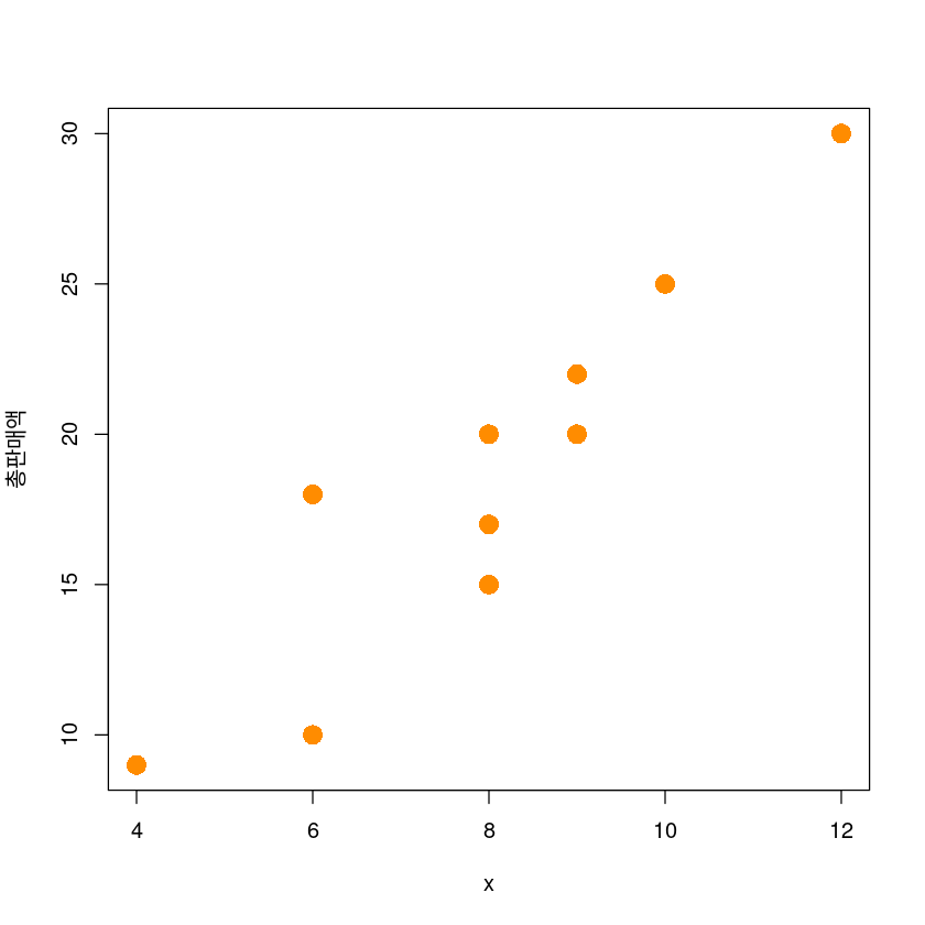
ggplot(dt, aes(x, y)) +
  geom_point(col='darkorange', size=3) +
  xlab("광고료")+ylab("총판매액")+
  theme_bw() +
  theme(axis.title = element_text(size = 14))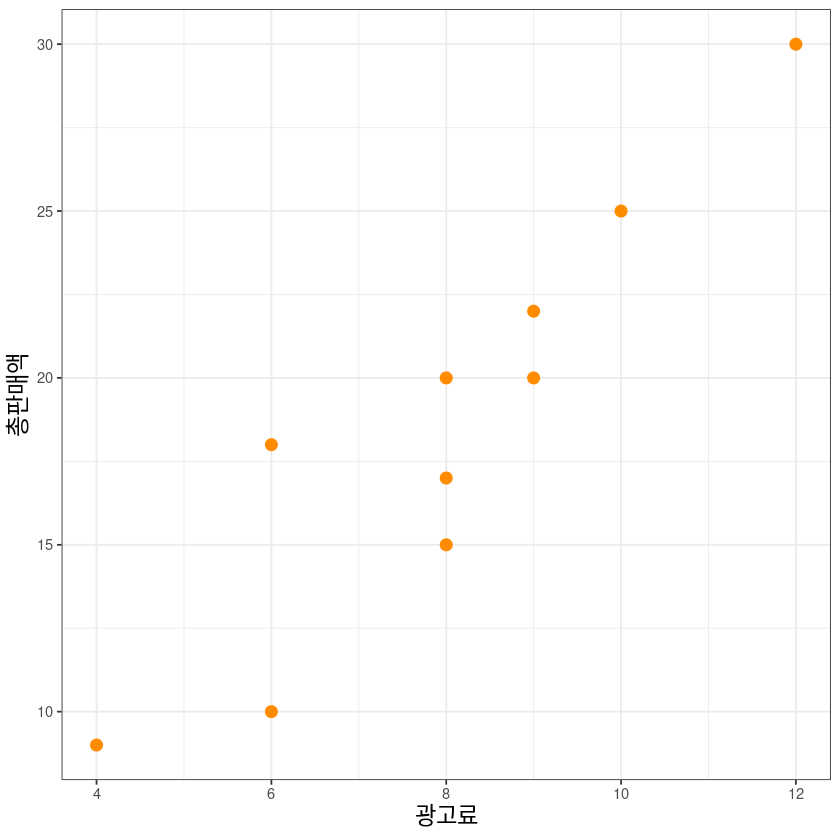
- 단순선형회귀모형 \[y= β_0 + β_1 x + ϵ\]
- 추정된 회귀직선
\[\widehat{y}=\widehat{E(y|X=x)}=\widehat{\beta_0}+\widehat{\beta_1}x\]
- 모형 적합
lm(formula, data)
formula: \(y=f(x)\), \(y\)(반응변수) ~ \(x\)(설명변수)
model1 <- lm(y~x, dt)- 직접계산
\[\widehat{\beta_0} = \bar y - \widehat{\beta_1} + \bar x \]
\[\widehat{\beta_1} = \dfrac{S_{xy}}{S_{xx}}\]
Sxy <-sum((dt$x - mean(dt$x))*(dt$y - mean(dt$y)))
Sxx <- sum((dt$x - mean(dt$x))^2)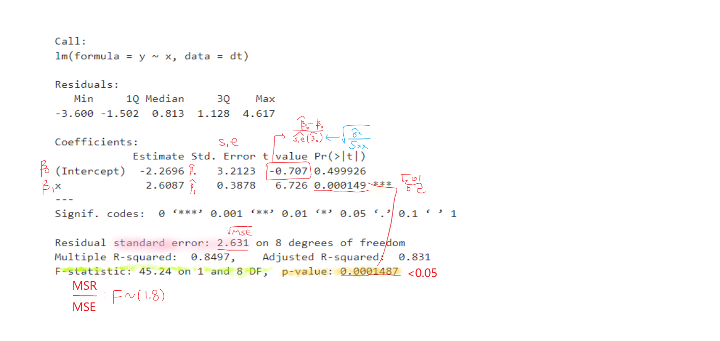
Sxy/Sxxsummary(model1)
Call:
lm(formula = y ~ x, data = dt)

Residuals:
   Min     1Q Median     3Q    Max
-3.600 -1.502  0.813  1.128  4.617

Coefficients:
            Estimate Std. Error t value Pr(>|t|)
(Intercept)  -2.2696     3.2123  -0.707 0.499926
x             2.6087     0.3878   6.726 0.000149 ***
---
Signif. codes:  0 ‘***’ 0.001 ‘**’ 0.01 ‘*’ 0.05 ‘.’ 0.1 ‘ ’ 1

Residual standard error: 2.631 on 8 degrees of freedom
Multiple R-squared:  0.8497,    Adjusted R-squared:  0.831
F-statistic: 45.24 on 1 and 8 DF,  p-value: 0.0001487
- summary
제일 먼저 F검정의 p-value값을 확인하자.
\(H_0\): \(\beta_1=0\) vs \(H_1\): not \(H_0\)
names(model1)model1$coefficients- 아래 값들은 모두 동일한 값을 리턴한다.
\[\widehat y = \widehat \beta_0 + \widehat \beta_1 x\]
model1$fitted.valuescoef(model1)[1] + coef(model1)[2]*dt$xfitted(model1)fitted.values(model1) - 아래 값들은 모두 동일한 값을 리턴한다.
\[e = y- \widehat y\]
model1$residualsdt$y - model1$fitted.valuesresid(model1)anova(model1)| Df | Sum Sq | Mean Sq | F value | Pr(>F) | |
|---|---|---|---|---|---|
| <int> | <dbl> | <dbl> | <dbl> | <dbl> | |
| x | 1 | 313.04348 | 313.043478 | 45.24034 | 0.0001486582 |
| Residuals | 8 | 55.35652 | 6.919565 | NA | NA |
a <- summary(model1)ls(a)a$r.squareda$adj.r.squareda$fstatistica$coef ## 회귀계수의 유의성 검정| Estimate | Std. Error | t value | Pr(>|t|) | |
|---|---|---|---|---|
| (Intercept) | -2.269565 | 3.212348 | -0.7065129 | 0.4999255886 |
| x | 2.608696 | 0.387847 | 6.7260939 | 0.0001486582 |
a$coef[,2] # s.econfint(model1, level=0.95)| 2.5 % | 97.5 % | |
|---|---|---|
| (Intercept) | -9.677252 | 5.138122 |
| x | 1.714319 | 3.503073 |
\[\widehat \beta \pm t_{\alpha/2}(n-2) s.e(\widehat \beta)\]
qt(0.025,8)qt(0.975,8) #왼쪽에 있는거 t_alpha/2 (n-2)coef(model1) + qt(0.975, 8) * summary(model1)$coef[,2]coef(model1) - qt(0.975, 8) * summary(model1)$coef[,2]\[y=\beta_1 x + \epsilon\]
model2 <- lm(y ~ 0 + x, dt)
summary(model2)
Call:
lm(formula = y ~ 0 + x, data = dt)

Residuals:
    Min      1Q  Median      3Q     Max
-4.0641 -1.5882  0.2638  1.4818  3.9359

Coefficients:
  Estimate Std. Error t value Pr(>|t|)
x   2.3440     0.0976   24.02  1.8e-09 ***
---
Signif. codes:  0 ‘***’ 0.001 ‘**’ 0.01 ‘*’ 0.05 ‘.’ 0.1 ‘ ’ 1

Residual standard error: 2.556 on 9 degrees of freedom
Multiple R-squared:  0.9846,    Adjusted R-squared:  0.9829
F-statistic: 576.8 on 1 and 9 DF, p-value: 1.798e-09summary(model1)$r.squared
summary(model2)$r.squaredanova(model2)| Df | Sum Sq | Mean Sq | F value | Pr(>F) | |
|---|---|---|---|---|---|
| <int> | <dbl> | <dbl> | <dbl> | <dbl> | |
| x | 1 | 3769.1895 | 3769.1895 | 576.8138 | 1.79763e-09 |
| Residuals | 9 | 58.8105 | 6.5345 | NA | NA |
dt1 <- data.frame(
  i = 1:nrow(dt),
  x = dt$x,
  y = dt$y,
  x_barx = dt$x - mean(dt$x),
y_bary = dt$y - mean(dt$y))dt1$x_barx2 <- dt1$x_barx^2
dt1$y_bary2 <- dt1$y_bary^2
dt1$xy <-dt1$x_barx * dt1$y_barydt1| i | x | y | x_barx | y_bary | x_barx2 | y_bary2 | xy |
|---|---|---|---|---|---|---|---|
| <int> | <dbl> | <dbl> | <dbl> | <dbl> | <dbl> | <dbl> | <dbl> |
| 1 | 4 | 9 | -4 | -9.6 | 16 | 92.16 | 38.4 |
| 2 | 8 | 20 | 0 | 1.4 | 0 | 1.96 | 0.0 |
| 3 | 9 | 22 | 1 | 3.4 | 1 | 11.56 | 3.4 |
| 4 | 8 | 15 | 0 | -3.6 | 0 | 12.96 | 0.0 |
| 5 | 8 | 17 | 0 | -1.6 | 0 | 2.56 | 0.0 |
| 6 | 12 | 30 | 4 | 11.4 | 16 | 129.96 | 45.6 |
| 7 | 6 | 18 | -2 | -0.6 | 4 | 0.36 | 1.2 |
| 8 | 10 | 25 | 2 | 6.4 | 4 | 40.96 | 12.8 |
| 9 | 6 | 10 | -2 | -8.6 | 4 | 73.96 | 17.2 |
| 10 | 9 | 20 | 1 | 1.4 | 1 | 1.96 | 1.4 |
round(colSums(dt1),3)- 직접계산
\[\widehat{\beta_0} = \bar y - \widehat{\beta_1} + \bar x \]
\[\widehat{\beta_1} = \dfrac{S_{xy}}{S_{xx}}\]
beta1 <- as.numeric(colSums(dt1)[8]/colSums(dt1)[6])

beta0 <- mean(dt$y) - beta1 * mean(dt$x)cat("hat beta0 = ", beta0)hat beta0 = -2.269565cat("hat beta1 = ", beta1)hat beta1 = 2.608696plot(y~x, data = dt,
xlab = "광고료",
ylab = "총판매액",
pch = 20,
cex = 2,
col = "darkorange",
ylim = c(0,35),
xlim = c(0, 12))
abline(model1, col='steelblue', lwd=2)
abline(model2, col='violet', lwd=2)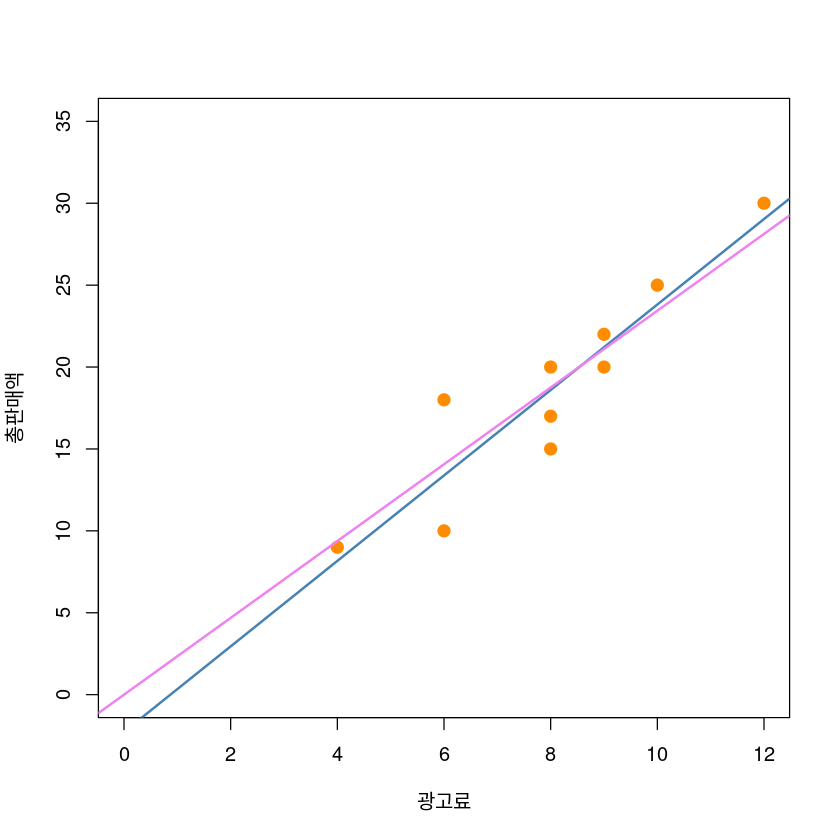
co <- coef(model1)
co_2 <- coef(model2) ggplot(dt, aes(x, y)) +
geom_point(col='steelblue', lwd=3) +
geom_abline(intercept = co[1], slope = co[2], col='darkorange', lwd=1) +
geom_abline(intercept = 0, slope = co_2, col='darkgreen', lwd=1) +
xlab("광고료")+ylab("총판매액")+
theme_bw()+
theme(axis.title = element_text(size = 16))Warning message in geom_point(col = "steelblue", lwd = 3):
“Ignoring unknown parameters: `linewidth`”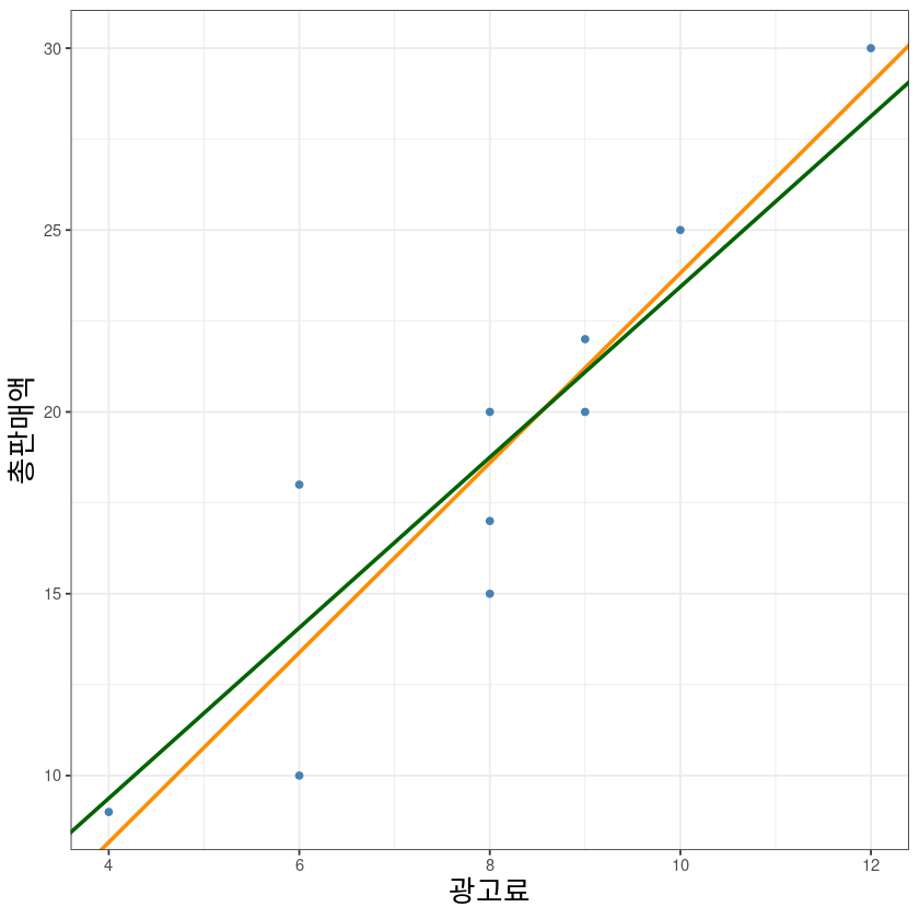
bb <- summary(model1)$sigma *
  sqrt( 1 + 1/10 + (dt$x - 8)^2/46) ## 개별 y에 대한 추정량의 표준오차
dt$ma95y <- model1$fitted + 2.306*bb
dt$mi95y <- model1$fitted - 2.306*bbqt(0.975,8)ggplot(dt, aes(x=x, y=y)) +
geom_point() +
geom_smooth(method=lm,
color="red", fill="#69b3a2", se=TRUE)+
geom_line(aes(x,mi95y), col='darkgrey', lty=2)+
geom_line(aes(x,ma95y), col='darkgrey', lty=2) +
theme_bw() +
theme(axis.title = element_blank())`geom_smooth()` using formula = 'y ~ x'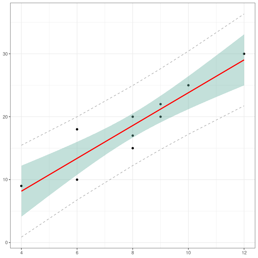
\[E(Y|x_0)\]
\[y=E(Y|x_0)+\epsilon\]
new_dt <- data.frame(x = 4.5)\[\widehat \mu_0 = \widehat y_0 = \widehat \beta_0 + \widehat \beta_1 4.5\]
model1$coefficients[1] + model1$coefficients[2]*4.5predict(model1, newdata = new_dt)predict(model1,
newdata = new_dt,
interval = c("confidence"), #구간추정
level = 0.95) ##평균반응| fit | lwr | upr | |
|---|---|---|---|
| 1 | 9.469565 | 5.79826 | 13.14087 |
predict(model1, newdata = new_dt,
        interval = c("prediction"),
level = 0.95) ## 개별 y| fit | lwr | upr | |
|---|---|---|---|
| 1 | 9.469565 | 2.379125 | 16.56001 |
dt_pred <- data.frame(
  x = c(1:12, 20, 35, 50),
  predict(model1,
          newdata=data.frame(x=c(1:12, 20, 35, 50)),
          interval="confidence", level = 0.95),
  predict(model1,
          newdata=data.frame(x=c(1:12, 20, 35, 50)),
          interval="prediction", level = 0.95)[,-1])
dt_pred| x | fit | lwr | upr | lwr.1 | upr.1 | |
|---|---|---|---|---|---|---|
| <dbl> | <dbl> | <dbl> | <dbl> | <dbl> | <dbl> | |
| 1 | 1 | 0.3391304 | -6.2087835 | 6.887044 | -8.5867330 | 9.264994 |
| 2 | 2 | 2.9478261 | -2.7509762 | 8.646628 | -5.3751666 | 11.270819 |
| 3 | 3 | 5.5565217 | 0.6905854 | 10.422458 | -2.2199297 | 13.332973 |
| 4 | 4 | 8.1652174 | 4.1058891 | 12.224546 | 0.8663128 | 15.464122 |
| 5 | 5 | 10.7739130 | 7.4756140 | 14.072212 | 3.8692308 | 17.678595 |
| 6 | 6 | 13.3826087 | 10.7597808 | 16.005437 | 6.7738957 | 19.991322 |
| 7 | 7 | 15.9913043 | 13.8748223 | 18.107786 | 9.5667143 | 22.415894 |
| 8 | 8 | 18.6000000 | 16.6817753 | 20.518225 | 12.2379683 | 24.962032 |
| 9 | 9 | 21.2086957 | 19.0922136 | 23.325178 | 14.7841056 | 27.633286 |
| 10 | 10 | 23.8173913 | 21.1945634 | 26.440219 | 17.2086783 | 30.426104 |
| 11 | 11 | 26.4260870 | 23.1277880 | 29.724386 | 19.5214047 | 33.330769 |
| 12 | 12 | 29.0347826 | 24.9754543 | 33.094111 | 21.7358781 | 36.333687 |
| 13 | 20 | 49.9043478 | 39.0017505 | 60.806945 | 37.4278703 | 62.380825 |
| 14 | 35 | 89.0347826 | 64.8105387 | 113.259027 | 64.0626010 | 114.006964 |
| 15 | 50 | 128.1652174 | 90.5524421 | 165.777993 | 90.0664414 | 166.263993 |
names(dt_pred)[5:6] <- c('plwr', 'pupr')
dt_pred| x | fit | lwr | upr | plwr | pupr | |
|---|---|---|---|---|---|---|
| <dbl> | <dbl> | <dbl> | <dbl> | <dbl> | <dbl> | |
| 1 | 1 | 0.3391304 | -6.2087835 | 6.887044 | -8.5867330 | 9.264994 |
| 2 | 2 | 2.9478261 | -2.7509762 | 8.646628 | -5.3751666 | 11.270819 |
| 3 | 3 | 5.5565217 | 0.6905854 | 10.422458 | -2.2199297 | 13.332973 |
| 4 | 4 | 8.1652174 | 4.1058891 | 12.224546 | 0.8663128 | 15.464122 |
| 5 | 5 | 10.7739130 | 7.4756140 | 14.072212 | 3.8692308 | 17.678595 |
| 6 | 6 | 13.3826087 | 10.7597808 | 16.005437 | 6.7738957 | 19.991322 |
| 7 | 7 | 15.9913043 | 13.8748223 | 18.107786 | 9.5667143 | 22.415894 |
| 8 | 8 | 18.6000000 | 16.6817753 | 20.518225 | 12.2379683 | 24.962032 |
| 9 | 9 | 21.2086957 | 19.0922136 | 23.325178 | 14.7841056 | 27.633286 |
| 10 | 10 | 23.8173913 | 21.1945634 | 26.440219 | 17.2086783 | 30.426104 |
| 11 | 11 | 26.4260870 | 23.1277880 | 29.724386 | 19.5214047 | 33.330769 |
| 12 | 12 | 29.0347826 | 24.9754543 | 33.094111 | 21.7358781 | 36.333687 |
| 13 | 20 | 49.9043478 | 39.0017505 | 60.806945 | 37.4278703 | 62.380825 |
| 14 | 35 | 89.0347826 | 64.8105387 | 113.259027 | 64.0626010 | 114.006964 |
| 15 | 50 | 128.1652174 | 90.5524421 | 165.777993 | 90.0664414 | 166.263993 |
barx <- mean(dt$x)
bary <- mean(dt$y)plot(y~x, data = dt,
xlab = "광고료",
ylab = "총판매액",
ylim = c(min(dt_pred$plwr), max(dt_pred$pupr)),
xlim = c(1,50),
pch = 20,
cex = 2,
col = "grey"
)
abline(model1, lwd = 5, col = "darkorange")
lines(dt_pred$x, dt_pred$lwr, col = "dodgerblue", lwd = 3, lty = 2)
lines(dt_pred$x, dt_pred$upr, col = "dodgerblue", lwd = 3, lty = 2)
lines(dt_pred$x, dt_pred$plwr, col = "darkgreen", lwd = 3, lty = 3)
lines(dt_pred$x, dt_pred$pupr, col = "darkgreen", lwd = 3, lty = 3)
abline(v=barx, lty=2, lwd=0.2, col='dark grey')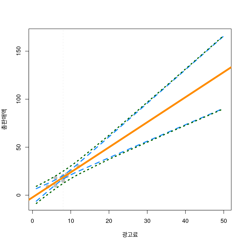
- \(\epsilon\) : 선형성, 등분산성, 정규성, 독립성
dt$yhat <- model1$fitted
dt$resid <- model1$residualspar(mfrow=c(1,2))
plot(resid ~ x, dt, pch=16, ylab = 'Residual')
abline(h=0, lty=2, col='grey')
plot(resid ~ yhat, dt, pch=16, ylab = 'Residual')
abline(h=0, lty=2, col='grey')
par(mfrow=c(1,1))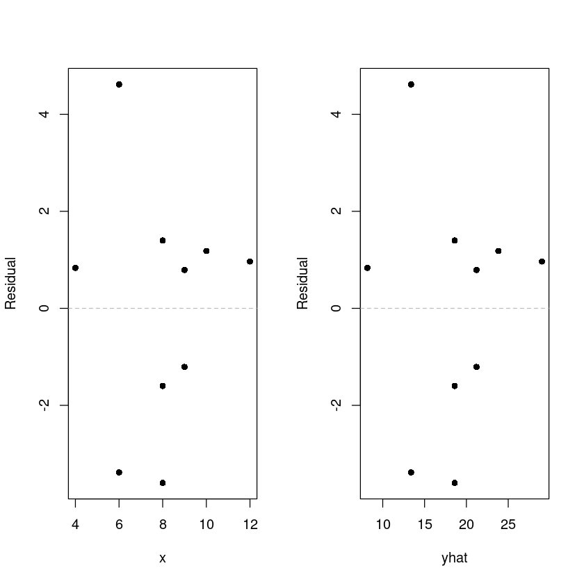
bptest(model1)
    studentized Breusch-Pagan test

data:  model1
BP = 1.6727, df = 1, p-value = 0.1959qqnorm(dt$resid, pch=16)
qqline(dt$resid, col = 2)
hist(dt$resid)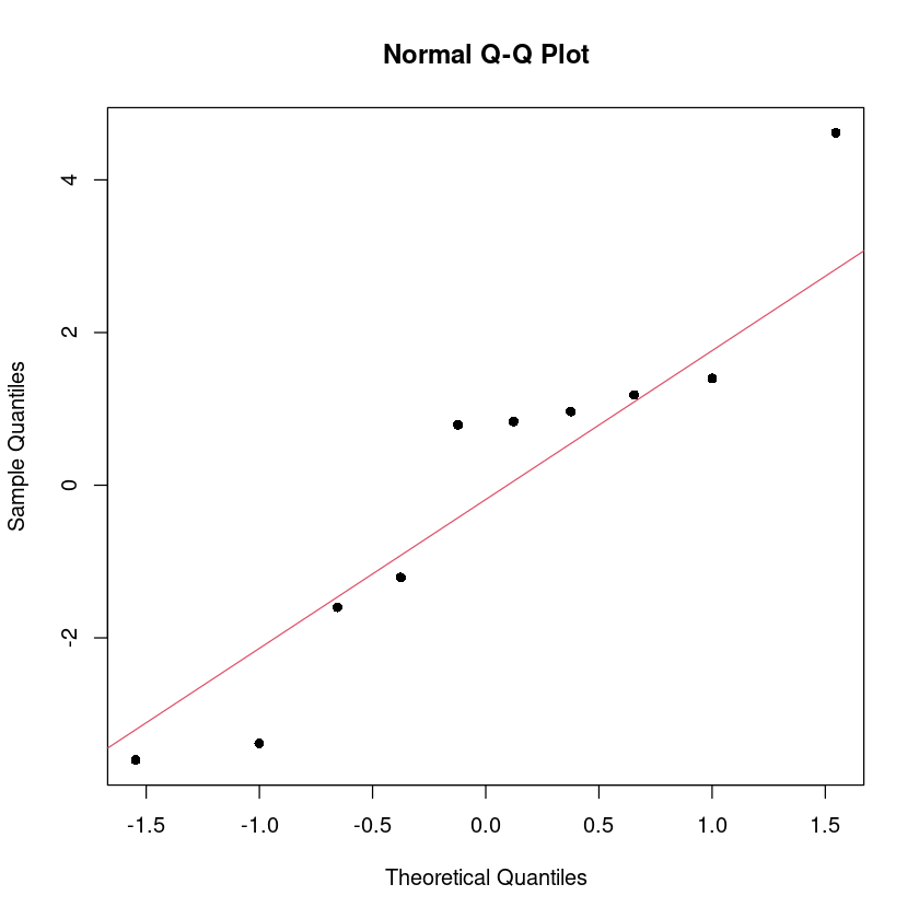
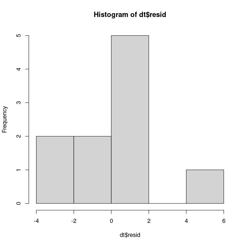
shapiro.test(resid(model1))
    Shapiro-Wilk normality test

data:  resid(model1)
W = 0.92426, p-value = 0.3939dwtest(model1, alternative = "two.sided") #H0 : uncorrelated vs H1 : rho != 0
    Durbin-Watson test

data:  model1
DW = 1.4679, p-value = 0.3916
alternative hypothesis: true autocorrelation is not 0dwtest(model1, alternative = "greater") #H0 : uncorrelated vs H1 : rho > 0
    Durbin-Watson test

data:  model1
DW = 1.4679, p-value = 0.1958
alternative hypothesis: true autocorrelation is greater than 0dwtest(model1, alternative = "less") #H0 : uncorrelated vs H1 : rho < 0
    Durbin-Watson test

data:  model1
DW = 1.4679, p-value = 0.8042
alternative hypothesis: true autocorrelation is less than 0