wind <- read.csv("wind.csv")
head(wind)| i | x | y | |
|---|---|---|---|
| <int> | <dbl> | <dbl> | |
| 1 | 1 | 5.0 | 1.582 |
| 2 | 2 | 6.0 | 1.822 |
| 3 | 3 | 3.4 | 1.057 |
| 4 | 4 | 2.7 | 0.500 |
| 5 | 5 | 10.0 | 2.236 |
| 6 | 6 | 9.7 | 2.386 |
해당 자료는 전북대학교 이영미 교수님 2023응용통계학 자료임
wind <- read.csv("wind.csv")
head(wind)| i | x | y | |
|---|---|---|---|
| <int> | <dbl> | <dbl> | |
| 1 | 1 | 5.0 | 1.582 |
| 2 | 2 | 6.0 | 1.822 |
| 3 | 3 | 3.4 | 1.057 |
| 4 | 4 | 2.7 | 0.500 |
| 5 | 5 | 10.0 | 2.236 |
| 6 | 6 | 9.7 | 2.386 |
par(mfrow=c(1,2))
plot(y~x, wind, pch=16, main="scatter plot")
abline(wind_fit, col='darkorange', lwd=2)

plot(fitted(wind_fit), rstandard(wind_fit),  pch = 16,
     xlab = expression(hat(y)),
     ylab = "Standardized Residuals",
     main = "Fitted vs. Residuals")
abline(h = 0, col = "grey", lwd = 2, lty=2)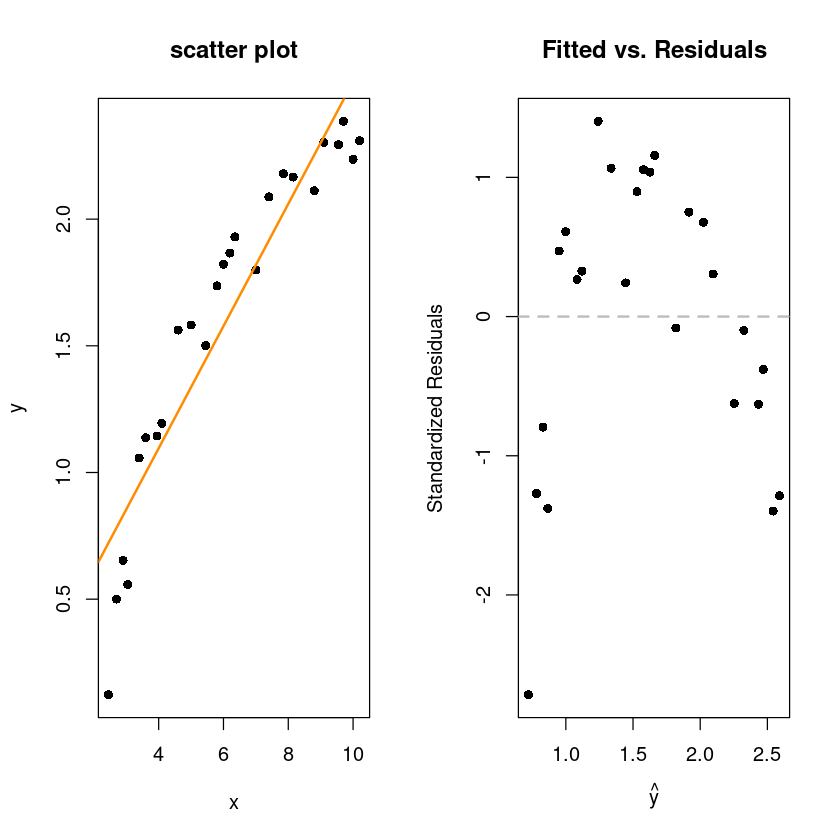
산점도를 봤을때 직선보다는 곡선이 어울려 보이는 산점도
표준화된잔차를 봐도 선형성(2차)이 보인다.
\(y=\beta_0+\beta_1x+\epsilon\)
wind_fit <- lm(y~x, wind)
summary(wind_fit)
Call:
lm(formula = y ~ x, data = wind)

Residuals:
     Min       1Q   Median       3Q      Max
-0.59869 -0.14099  0.06059  0.17262  0.32184

Coefficients:
            Estimate Std. Error t value Pr(>|t|)
(Intercept)  0.13088    0.12599   1.039     0.31
x            0.24115    0.01905  12.659 7.55e-12 ***
---
Signif. codes:  0 ‘***’ 0.001 ‘**’ 0.01 ‘*’ 0.05 ‘.’ 0.1 ‘ ’ 1

Residual standard error: 0.2361 on 23 degrees of freedom
Multiple R-squared:  0.8745,    Adjusted R-squared:  0.869
F-statistic: 160.3 on 1 and 23 DF, p-value: 7.546e-12print(paste0("coefficient of determination : ", round(summary(wind_fit)$r.squared,3)))[1] "coefficient of determination : 0.874"print(paste0("RMSE : ", round(summary(wind_fit)$sigma,3)))[1] "RMSE : 0.236"\(y=\beta_0+\beta_1x+\beta_2x^2+\epsilon\)
wind_fit_2 <- lm(y~x+I(x^2), wind)
summary(wind_fit_2)
Call:
lm(formula = y ~ x + I(x^2), data = wind)

Residuals:
     Min       1Q   Median       3Q      Max
-0.26347 -0.02537  0.01264  0.03908  0.19903

Coefficients:
             Estimate Std. Error t value Pr(>|t|)
(Intercept) -1.155898   0.174650  -6.618 1.18e-06 ***
x            0.722936   0.061425  11.769 5.77e-11 ***
I(x^2)      -0.038121   0.004797  -7.947 6.59e-08 ***
---
Signif. codes:  0 ‘***’ 0.001 ‘**’ 0.01 ‘*’ 0.05 ‘.’ 0.1 ‘ ’ 1

Residual standard error: 0.1227 on 22 degrees of freedom
Multiple R-squared:  0.9676,    Adjusted R-squared:  0.9646
F-statistic: 328.3 on 2 and 22 DF, p-value: < 2.2e-16\(x^2\)을 넣었더니 모형도 유의하고 \(R^2\)의 값도 커짐
두개 변수 모두 유의함
par(mfrow=c(1,2))
plot(y~x, wind, pch=16, main="scatter plot")
x_new <- sort(wind$x)
lines(x_new, predict(wind_fit_2, newdata = data.frame(x=x_new)), col='darkorange', lwd=2)

plot(fitted(wind_fit_2), rstandard(wind_fit_2),  pch = 16,
      xlab = expression(hat(y)),
      ylab = "Standardized Residuals",
      main = "Fitted vs. Residuals")
abline(h = 0, col = "grey", lwd = 2, lty=2)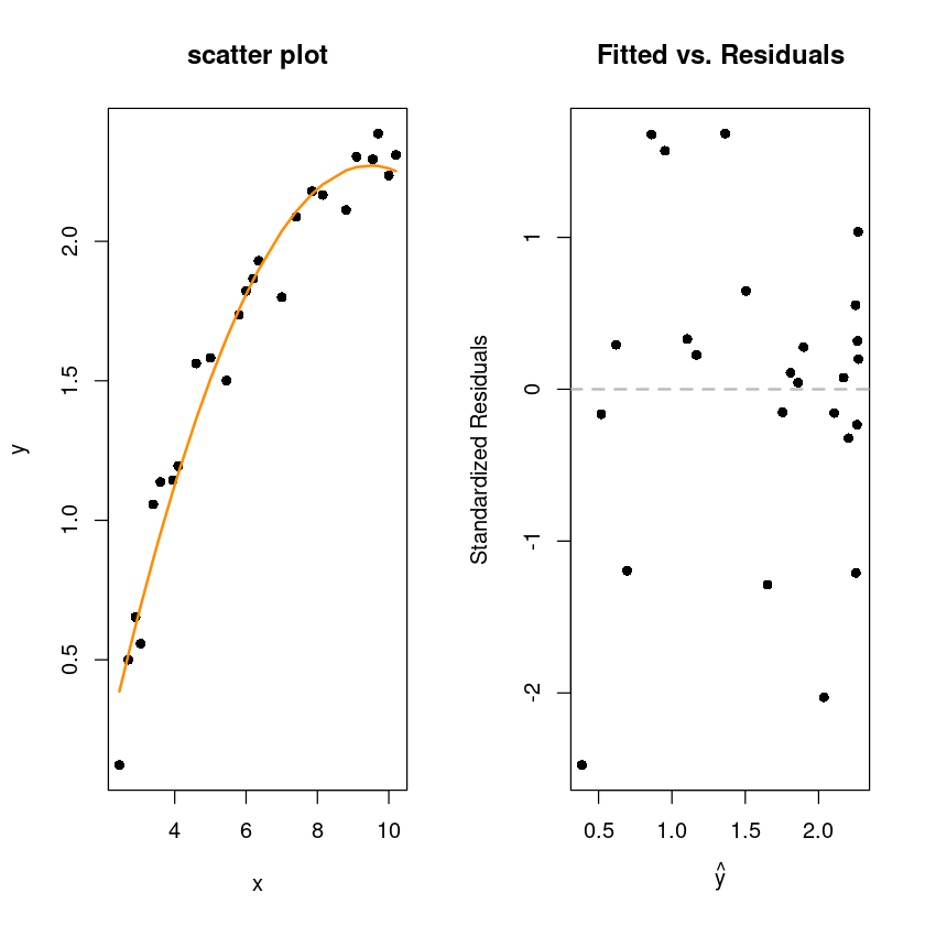
print(paste0("coefficient of determination : ", round(summary(wind_fit_2)$r.squared,3)))[1] "coefficient of determination : 0.968"print(paste0("RMSE : ", round(summary(wind_fit_2)$sigma,3)))[1] "RMSE : 0.123"\(y=\beta_0+\beta_1 \dfrac{1}{x}+\epsilon=\beta_0+\beta_1 x^`+\epsilon\)
wind_fit_3 <- lm(y~I(1/x), wind)
summary(wind_fit_3)
Call:
lm(formula = y ~ I(1/x), data = wind)

Residuals:
     Min       1Q   Median       3Q      Max
-0.20547 -0.04940  0.01100  0.08352  0.12204

Coefficients:
            Estimate Std. Error t value Pr(>|t|)
(Intercept)   2.9789     0.0449   66.34   <2e-16 ***
I(1/x)       -6.9345     0.2064  -33.59   <2e-16 ***
---
Signif. codes:  0 ‘***’ 0.001 ‘**’ 0.01 ‘*’ 0.05 ‘.’ 0.1 ‘ ’ 1

Residual standard error: 0.09417 on 23 degrees of freedom
Multiple R-squared:   0.98, Adjusted R-squared:  0.9792
F-statistic: 1128 on 1 and 23 DF, p-value: < 2.2e-16par(mfrow=c(1,2))
plot(y~I(1/x), wind, pch=16, main="scatter plot")
abline(wind_fit_3, col='darkorange', lwd=2)
plot(fitted(wind_fit_3), rstandard(wind_fit_3), pch = 16,
xlab = expression(hat(y)),
ylab = "Standardized Residuals",
main = "Fitted vs. Residuals")
abline(h = 0, col = "grey", lwd = 2, lty=2)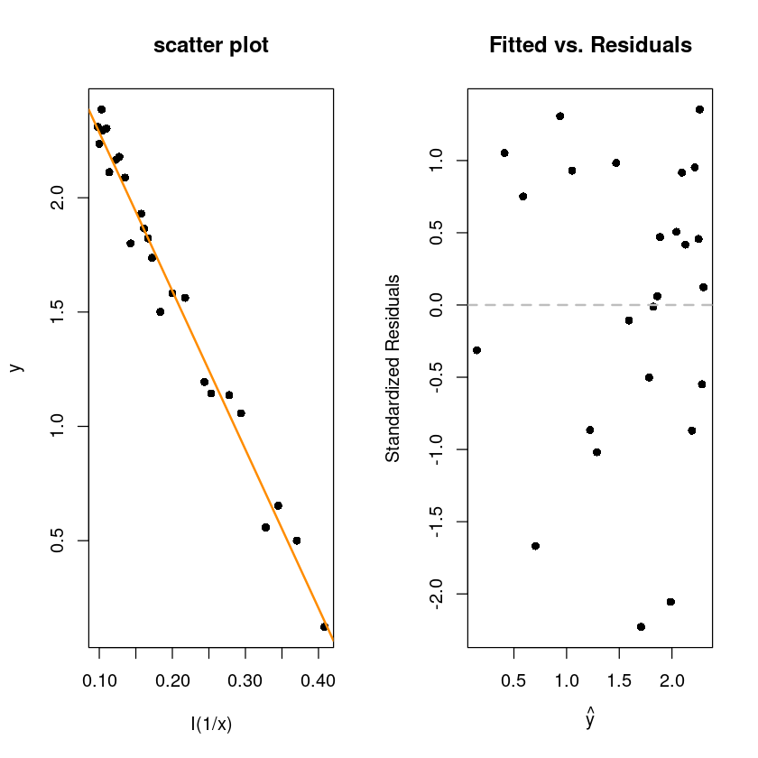
print(paste0("coefficient of determination : ", round(summary(wind_fit_3)$r.squared,3)))[1] "coefficient of determination : 0.98"print(paste0("RMSE : ", round(summary(wind_fit_3)$sigma,3)))[1] "RMSE : 0.094"initech <- read.csv("initech.csv")
head(initech)| years | salary | |
|---|---|---|
| <int> | <int> | |
| 1 | 1 | 41504 |
| 2 | 1 | 32619 |
| 3 | 1 | 44322 |
| 4 | 2 | 40038 |
| 5 | 2 | 46147 |
| 6 | 2 | 38447 |
par(mfrow=c(1,1))
plot(salary~years, initech,  pch=16, cex=1.5)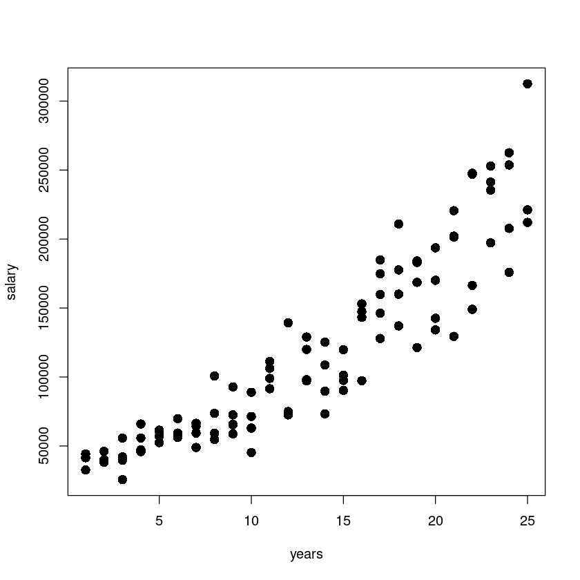
곡선 관계!?
x가 증가하면서 y값이 점점 퍼지고 있다. x가 증가할수록 salary의 분산이 커지고 있다.
\(y=\beta_0+\beta_x+\epsilon\)
initech_fit <- lm(salary~years, initech)
summary(initech_fit)
Call:
lm(formula = salary ~ years, data = initech)

Residuals:
   Min     1Q Median     3Q    Max
-57225 -18104    241  15589  91332

Coefficients:
            Estimate Std. Error t value Pr(>|t|)
(Intercept)     5302       5750   0.922    0.359
years           8637        389  22.200   <2e-16 ***
---
Signif. codes:  0 ‘***’ 0.001 ‘**’ 0.01 ‘*’ 0.05 ‘.’ 0.1 ‘ ’ 1

Residual standard error: 27360 on 98 degrees of freedom
Multiple R-squared:  0.8341,    Adjusted R-squared:  0.8324
F-statistic: 492.8 on 1 and 98 DF, p-value: < 2.2e-16plot(salary~years, initech,
pch=16, cex=1.5)
abline(initech_fit, col='darkorange', lwd=2)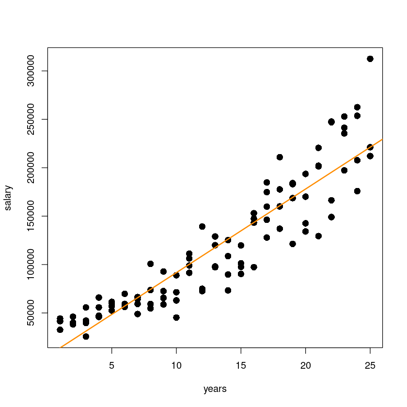
par(mfrow=c(1,2))

plot(fitted(initech_fit), rstandard(initech_fit),  pch = 16,
     xlab = expression(hat(y)),
     ylab = "Standardized Residuals",
     main = "Fitted versus Residuals")
abline(h = 0, col = "grey", lwd = 2, lty=2)

qqnorm(resid(initech_fit), pch=16,
          main = "Normal Q-Q Plot", col = "darkgrey")
qqline(resid(initech_fit), col = "dodgerblue", lwd = 2)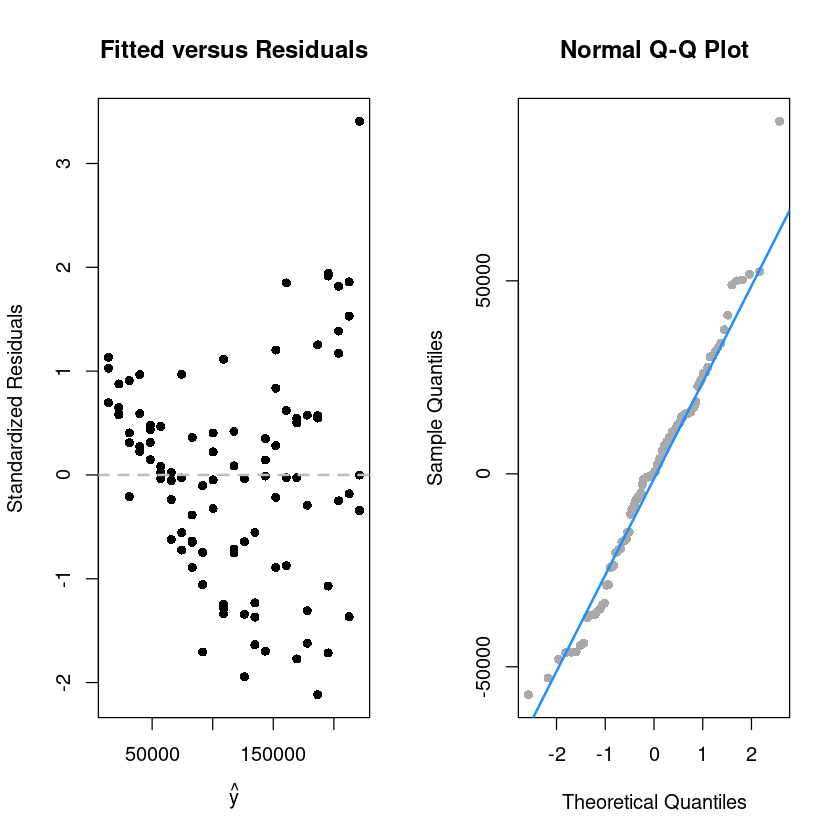
library(lmtest)Loading required package: zoo
Attaching package: ‘zoo’
The following objects are masked from ‘package:base’:
as.Date, as.Date.numeric
dwtest(initech_fit, alternative = "two.sided")
    Durbin-Watson test

data:  initech_fit
DW = 1.3313, p-value = 0.0004993
alternative hypothesis: true autocorrelation is not 0
등분산성 만족하지 않는다.
변수변환(log y),WLSE -> GLS 를 한다.
hist(resid(initech_fit))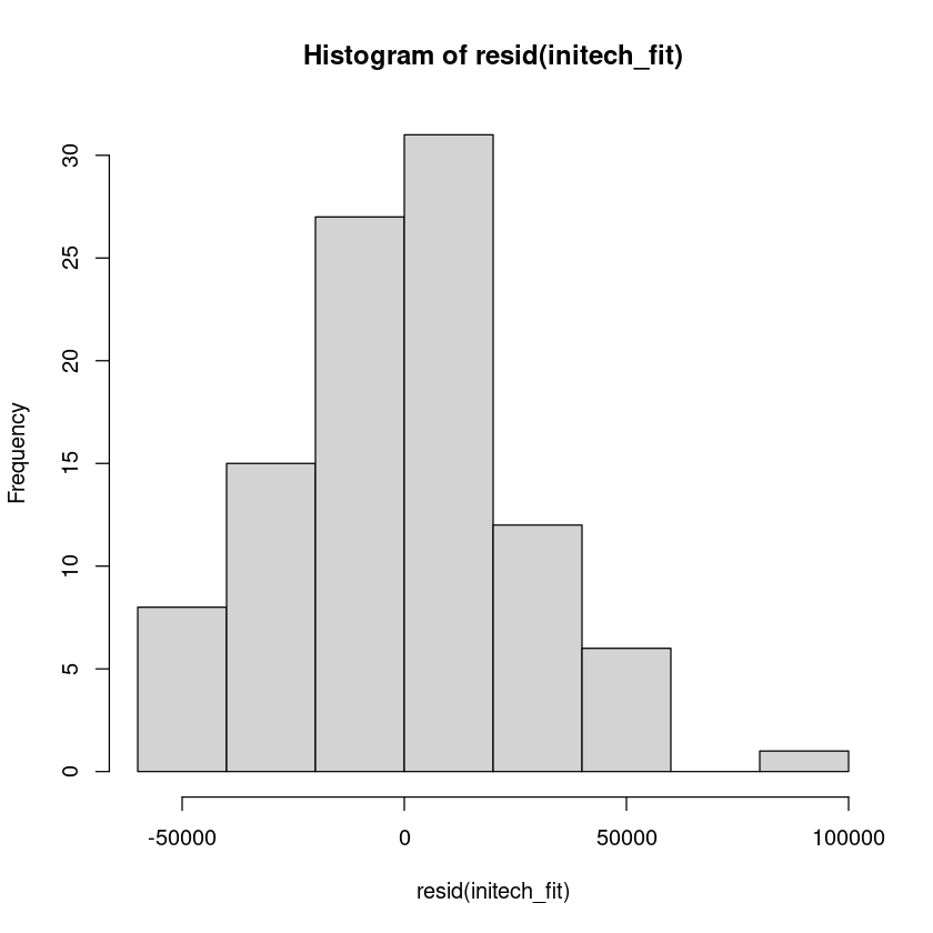
initech_fit_log = lm(log(salary) ~ years, data = initech)
summary(initech_fit_log)
Call:
lm(formula = log(salary) ~ years, data = initech)

Residuals:
     Min       1Q   Median       3Q      Max
-0.57022 -0.13560  0.03048  0.14157  0.41366

Coefficients:
            Estimate Std. Error t value Pr(>|t|)
(Intercept) 10.48381    0.04108  255.18   <2e-16 ***
years        0.07888    0.00278   28.38   <2e-16 ***
---
Signif. codes:  0 ‘***’ 0.001 ‘**’ 0.01 ‘*’ 0.05 ‘.’ 0.1 ‘ ’ 1

Residual standard error: 0.1955 on 98 degrees of freedom
Multiple R-squared:  0.8915,    Adjusted R-squared:  0.8904
F-statistic: 805.2 on 1 and 98 DF,  p-value: < 2.2e-16
로그변환을 한 모형이므로 RMSE가 작다고 엇 작네 하면 안돼 .y를 예측하는 것과 y`을 예측하는것은 다르다.
\(log \hat y = \hat y^` = \hat \beta_0 + \hat \beta_1 x_1\)
\(\rightarrow \hat y = exp(\hat y^`)\) 역변환 해줘야함
par(mfrow=c(1,2))
plot(log(salary)~years, initech,
        pch=16, cex=1.5)
abline(initech_fit_log, col='darkorange', lwd=2)

plot(salary~years, initech,pch=16, cex=1.5)
lines(initech$years,exp(fitted(initech_fit_log)), col="darkorange", lwd=2)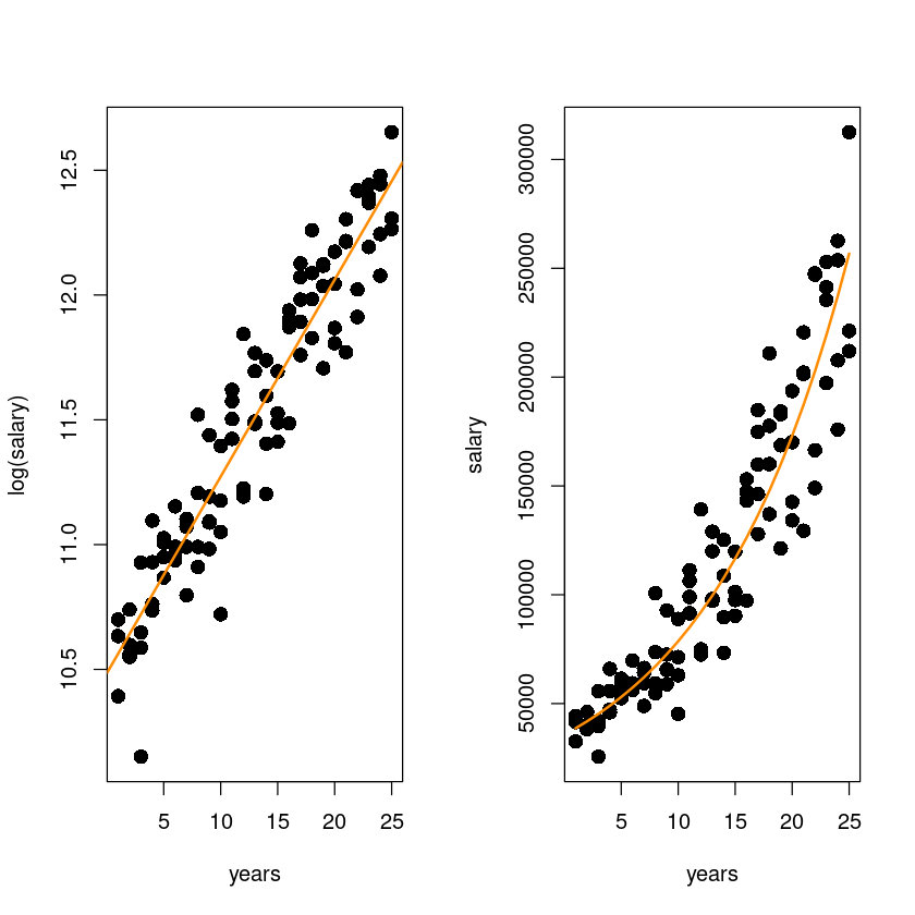
왼쪽 그림: \(\hat y^` = \hat {log y}\)
오른쪽 그림: \(\hat y = exp(\hat \beta_0 + \hat \beta_1x)\)
par(mfrow=c(1,2))

plot(fitted(initech_fit_log), rstandard(initech_fit_log),  pch = 16,
     xlab = expression(hat(y)),
     ylab = "Standardized Residuals",
     main = "Fitted versus Residuals")
abline(h = 0, col = "grey", lwd = 2, lty=2)

qqnorm(resid(initech_fit_log), pch=16,
          main = "Normal Q-Q Plot", col = "darkgrey")
qqline(resid(initech_fit_log), col = "dodgerblue", lwd = 2)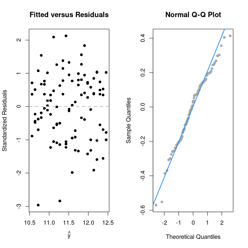
\(y=\beta_0+\beta_x+\epsilon\)
summary(initech_fit)$sigma\(log y = \beta_0+\beta_1x+\epsilon\)
summary(initech_fit_log)$sigma\(\sqrt{MSE}=\hat \sigma\) -LM1
sqrt(sum((initech$salary - fitted(initech_fit)) ^ 2)/98) \(\sqrt{MSE}=\hat \sigma\) -LM2
sqrt(sum((initech$salary - exp(fitted(initech_fit_log))) ^ 2)/98)\(y-(exp(\hat{log y})=\hat y)\)
\(y'=log y\)
log변환은 앞쪽은 작게 압축시키고 뒤쪽은 확 압축시킴
log변환과 다르게 덜 압축하는 방법??? sqrt로 압축..
지수변환 \(\lambda\)파라미터를 이용해서 변환.. (일반화..)
\[y'=g_{\lambda}(y)= \begin{cases} \dfrac{y^{\lambda}-1}{\lambda} & \lambda \neq 0 \\ log y & \lambda=0 \end{cases}\]
library(MASS)
boxcox(initech_fit, plotit = TRUE)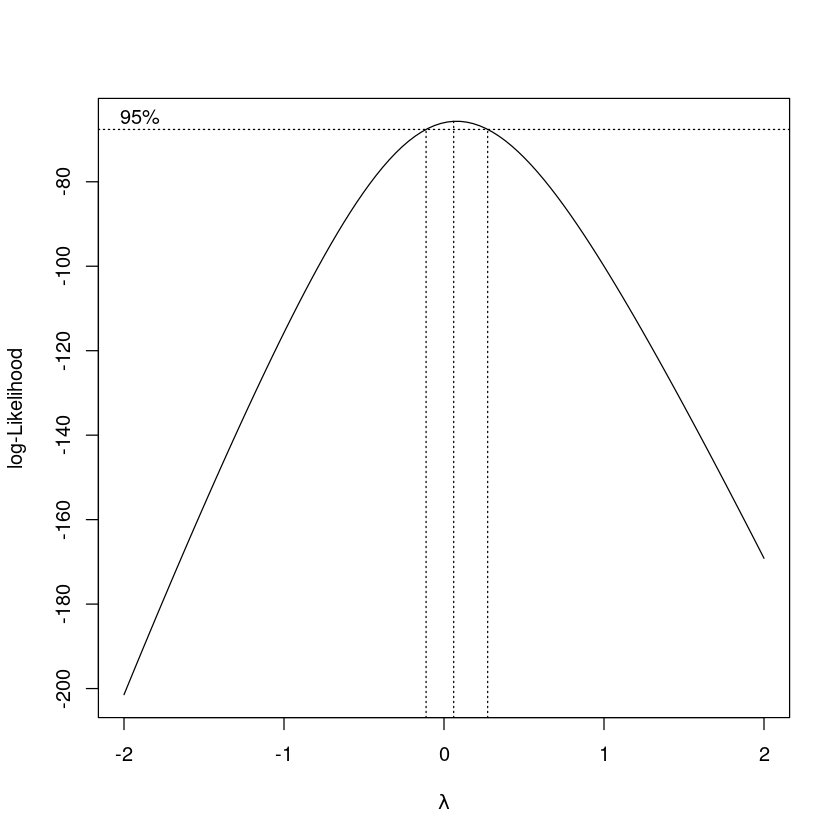
(-2,2)가 기본으로 보여줌
0을 좌우로 점선은 \(\lambda\)의 95% 신뢰구간
boxcox(initech_fit, plotit = TRUE, lambda = seq(-0.5,0.5, by = 0.1))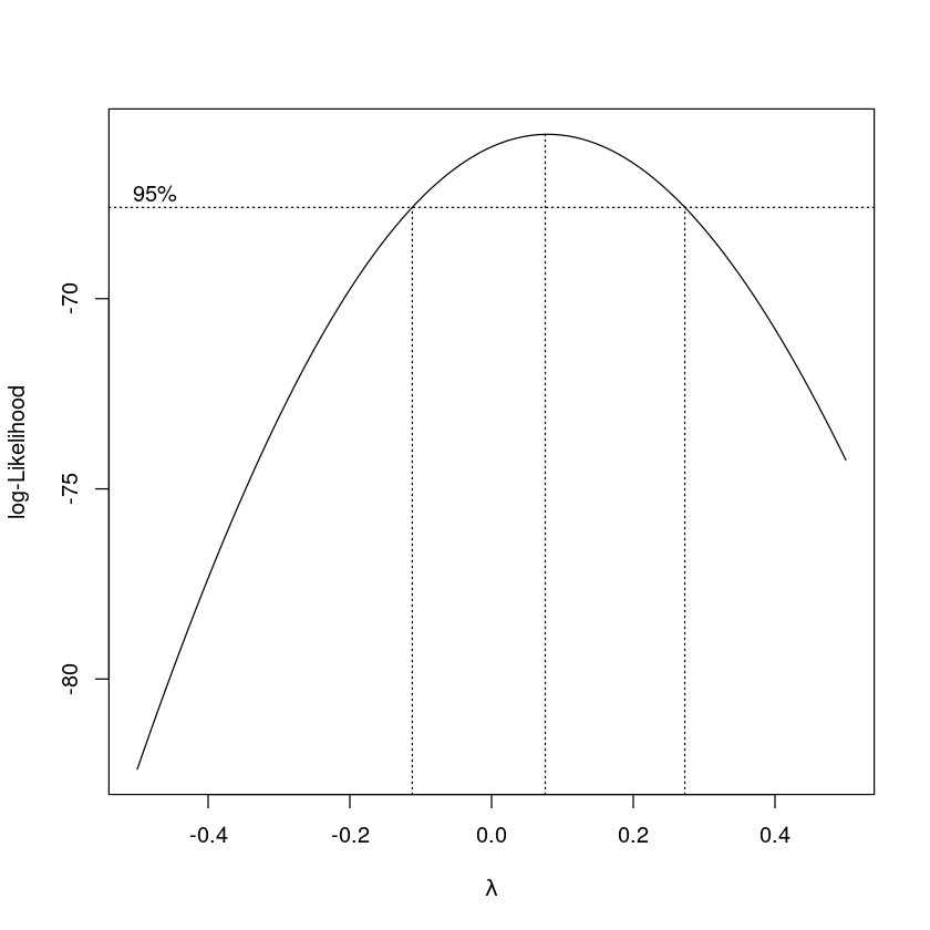
log-Likeilihood를 이용하여 가장 큰 \(\lambda\)를 찾아준다.
\(\lambda\)를 결정해주는 함수->boxcox
가장 큰 \(\hat \lambda\) 은 0.08… 근데 의미가 없음.. 신뢰구간에 0이 들어가있네? 0은 로그변환이니까 0도 괜찮겠다!