library(MASS) #lm.ridge
library(car) #vif해당 자료는 전북대학교 이영미 교수님 2023응용통계학 자료임
library(glmnet) #Ridge, LassoLoading required package: Matrix
Loaded glmnet 4.1-7
완전한 다중공선성 (perfect multicollinearity)
완전한 다중공산성을 갖는 데이터 생성
gen_perfect_collin_data = function(num_samples = 100) {
     x1 = rnorm(n = num_samples, mean = 80, sd = 10)
     x2 = rnorm(n = num_samples, mean = 70, sd = 5)
     x3 = 2 * x1 + 4 * x2 + 3
     y = 3 + x1 + x2 + rnorm(n = num_samples, mean = 0, sd = 1)
    data.frame(y, x1, x2, x3)
    }
x1과 x2는 independent
x3는 선형결합
set.seed(42)
perfect_collin_data = gen_perfect_collin_data()
head(perfect_collin_data)| y | x1 | x2 | x3 | |
|---|---|---|---|---|
| <dbl> | <dbl> | <dbl> | <dbl> | |
| 1 | 170.7135 | 93.70958 | 76.00483 | 494.4385 |
| 2 | 152.9106 | 74.35302 | 75.22376 | 452.6011 |
| 3 | 152.7866 | 83.63128 | 64.98396 | 430.1984 |
| 4 | 170.6306 | 86.32863 | 79.24241 | 492.6269 |
| 5 | 152.3320 | 84.04268 | 66.66613 | 437.7499 |
| 6 | 151.3155 | 78.93875 | 70.52757 | 442.9878 |
round(cor(perfect_collin_data),4)| y | x1 | x2 | x3 | |
|---|---|---|---|---|
| y | 1.0000 | 0.9112 | 0.4307 | 0.9558 |
| x1 | 0.9112 | 1.0000 | 0.0313 | 0.7639 |
| x2 | 0.4307 | 0.0313 | 1.0000 | 0.6690 |
| x3 | 0.9558 | 0.7639 | 0.6690 | 1.0000 |
perfect_collin_fit = lm(y ~ x1 + x2 + x3, data = perfect_collin_data)
summary(perfect_collin_fit)
Call:
lm(formula = y ~ x1 + x2 + x3, data = perfect_collin_data)

Residuals:
     Min       1Q   Median       3Q      Max
-2.57662 -0.66188 -0.08253  0.63706  2.52057

Coefficients: (1 not defined because of singularities)
            Estimate Std. Error t value Pr(>|t|)
(Intercept) 2.957336   1.735165   1.704   0.0915 .
x1          0.985629   0.009788 100.702   <2e-16 ***
x2          1.017059   0.022545  45.112   <2e-16 ***
x3                NA         NA      NA       NA
---
Signif. codes:  0 ‘***’ 0.001 ‘**’ 0.01 ‘*’ 0.05 ‘.’ 0.1 ‘ ’ 1

Residual standard error: 1.014 on 97 degrees of freedom
Multiple R-squared:  0.9923,    Adjusted R-squared:  0.9921
F-statistic:  6236 on 2 and 97 DF,  p-value: < 2.2e-16
p-value값 유의하게 나오고, \(R^2\)값도 크다.
\(rank(X)=3\)(x3가 x1과 x2의 선형결합으로 이루어진 변수이므로)
\(\rightarrow (X^TX)^{-1}\)값을 구할 수 없으므로 \(\hat \beta\)값을 구할 수 없다. 그래서 R에서는 한 개의 변수를 빼고 lm을 돌린다.
fit1 = lm(y ~ x1 + x2, data = perfect_collin_data)
fit2 = lm(y ~ x1 + x3, data = perfect_collin_data)
fit3 = lm(y ~ x2 + x3, data = perfect_collin_data)
- x3는 선형결합으로 이루어진 변수이므로 위 예시에서 두 개의 변수만 안다는 것은 세 개의 변수를 안다는 것과 동치
summary(fit1)
Call:
lm(formula = y ~ x1 + x2, data = perfect_collin_data)

Residuals:
     Min       1Q   Median       3Q      Max
-2.57662 -0.66188 -0.08253  0.63706  2.52057

Coefficients:
            Estimate Std. Error t value Pr(>|t|)
(Intercept) 2.957336   1.735165   1.704   0.0915 .
x1          0.985629   0.009788 100.702   <2e-16 ***
x2          1.017059   0.022545  45.112   <2e-16 ***
---
Signif. codes:  0 ‘***’ 0.001 ‘**’ 0.01 ‘*’ 0.05 ‘.’ 0.1 ‘ ’ 1

Residual standard error: 1.014 on 97 degrees of freedom
Multiple R-squared:  0.9923,    Adjusted R-squared:  0.9921
F-statistic: 6236 on 2 and 97 DF, p-value: < 2.2e-16summary(fit2)
Call:
lm(formula = y ~ x1 + x3, data = perfect_collin_data)

Residuals:
     Min       1Q   Median       3Q      Max
-2.57662 -0.66188 -0.08253  0.63706  2.52057

Coefficients:
            Estimate Std. Error t value Pr(>|t|)
(Intercept) 2.194542   1.750225   1.254    0.213
x1          0.477100   0.015158  31.475   <2e-16 ***
x3          0.254265   0.005636  45.112   <2e-16 ***
---
Signif. codes:  0 ‘***’ 0.001 ‘**’ 0.01 ‘*’ 0.05 ‘.’ 0.1 ‘ ’ 1

Residual standard error: 1.014 on 97 degrees of freedom
Multiple R-squared:  0.9923,    Adjusted R-squared:  0.9921
F-statistic:  6236 on 2 and 97 DF,  p-value: < 2.2e-16
\(y=\beta_0 + \beta_1x_1 + \beta_2 x_3 + \epsilon\)
\(x_3 = 2x_1+4x_2+3\) 대입
\(y=\beta_0 +\beta_1x_1 + 2\beta_2x_1 + 4\beta_2 x_2 + 3\beta_2 = (\beta_0 + 3\beta_2)+(\beta_1+2\beta_2)x_1 + 4\beta_2 x_2\)
계수가 좀 달라지지만 x1과 x2의 식으로 다시 써질 수 있음
summary(fit3)
Call:
lm(formula = y ~ x2 + x3, data = perfect_collin_data)

Residuals:
     Min       1Q   Median       3Q      Max
-2.57662 -0.66188 -0.08253  0.63706  2.52057

Coefficients:
             Estimate Std. Error t value Pr(>|t|)
(Intercept)  1.478892   1.741452   0.849    0.398
x2          -0.954200   0.030316 -31.475   <2e-16 ***
x3           0.492815   0.004894 100.702   <2e-16 ***
---
Signif. codes:  0 ‘***’ 0.001 ‘**’ 0.01 ‘*’ 0.05 ‘.’ 0.1 ‘ ’ 1

Residual standard error: 1.014 on 97 degrees of freedom
Multiple R-squared:  0.9923,    Adjusted R-squared:  0.9921
F-statistic: 6236 on 2 and 97 DF, p-value: < 2.2e-16- fit1, fit2, fit3의 \(R^2\)가 다 똑같다. 모형의 적합도가 동일하다.
all.equal(fitted(fit1), fitted(fit2))
TRUE
all.equal(fitted(fit2), fitted(fit3))
TRUE
all.equal: 동일한 함수이냐?
coef(fit1)- (Intercept)
- 2.95733574182587
- x1
- 0.985629075384886
- x2
- 1.01705863569558
coef(fit2)- (Intercept)
- 2.19454176505435
- x1
- 0.477099757537094
- x3
- 0.254264658923896
coef(fit3)- (Intercept)
- 1.47889212874879
- x2
- -0.954199515074186
- x3
- 0.492814537692442
완전에 가까운 다중공선성 (approximate multicollinearity)
완전에 가까운 다중공선성을 갖는 데이터 생성
gen_almost_collin_data = function(num_samples = 100) {
    x1 = rnorm(n = num_samples, mean = 0, sd = 2)
    x2 = rnorm(n = num_samples, mean = 0, sd = 3)
    x3 = 3*x1 + 1*x2 + rnorm(num_samples, mean=0, sd=0.5)
    y = 3 + x1 + x2 + rnorm(n = num_samples, mean = 0, sd = 1)
    data.frame(y, x1, x2, x3)
}- rank(X)=4가 된다. 약간의 noise가 있음
set.seed(42)
almost_collin_data = gen_almost_collin_data()
head(almost_collin_data)| y | x1 | x2 | x3 | |
|---|---|---|---|---|
| <dbl> | <dbl> | <dbl> | <dbl> | |
| 1 | 9.3401923 | 2.7419169 | 3.6028961 | 10.82818219 |
| 2 | 5.7650991 | -1.1293963 | 3.1342533 | -0.08704717 |
| 3 | 0.7556218 | 0.7262568 | -3.0096259 | -0.24519291 |
| 4 | 10.5462431 | 1.2657252 | 5.5454457 | 10.37239096 |
| 5 | 1.6617438 | 0.8085366 | -2.0003202 | -0.26314109 |
| 6 | 3.0464051 | -0.2122490 | 0.3165414 | -0.89563344 |
round(cor(almost_collin_data),3)| y | x1 | x2 | x3 | |
|---|---|---|---|---|
| y | 1.000 | 0.616 | 0.769 | 0.863 |
| x1 | 0.616 | 1.000 | 0.031 | 0.913 |
| x2 | 0.769 | 0.031 | 1.000 | 0.429 |
| x3 | 0.863 | 0.913 | 0.429 | 1.000 |
m <- lm(y~., almost_collin_data) summary(m)
Call:
lm(formula = y ~ ., data = almost_collin_data)

Residuals:
    Min      1Q  Median      3Q     Max
-1.7944 -0.5867 -0.1038  0.6188  2.3280

Coefficients:
            Estimate Std. Error t value Pr(>|t|)
(Intercept)  3.03150    0.08914  34.007  < 2e-16 ***
x1           1.21854    0.52829   2.307   0.0232 *
x2           1.06616    0.18314   5.821 7.71e-08 ***
x3          -0.06322    0.17765  -0.356   0.7227
---
Signif. codes:  0 ‘***’ 0.001 ‘**’ 0.01 ‘*’ 0.05 ‘.’ 0.1 ‘ ’ 1

Residual standard error: 0.8867 on 96 degrees of freedom
Multiple R-squared:  0.9419,    Adjusted R-squared:  0.9401
F-statistic:   519 on 3 and 96 DF,  p-value: < 2.2e-16
모형은 유의하고, \(R^2\)값도 큰 편
설명변수들은 별로 유의하지 않다.(x1과 x3).. 다중공산성이 있기 떄문에
위의 fit3와 비교해보면, std.Error값이 많이 커진 것을 볼 수 있음. x2의 std.Error값 (0.03 -> 0.183) x3의 std.Error값 (0.005 -> 0.1777)
vif(m)- x1
- 152.426839030633
- x2
- 31.0734919101693
- x3
- 186.719994280627
vif>10 이면 다중공산성이 있다.
Std. Error값이 커진다. -> 불안정해짐. 과녁중앙에서 벗어나게..
- y에 noise
set.seed(1000)
noise <- rnorm(n = 100, mean = 0, sd =0.5)
m_noise <- lm(y+noise~., almost_collin_data)
summary(m_noise)
Call:
lm(formula = y + noise ~ ., data = almost_collin_data)

Residuals:
    Min      1Q  Median      3Q     Max
-2.0962 -0.6998 -0.0891  0.7726  2.8462

Coefficients:
            Estimate Std. Error t value Pr(>|t|)
(Intercept)   3.0403     0.1020  29.815  < 2e-16 ***
x1            0.9894     0.6043   1.637    0.105
x2            0.9898     0.2095   4.725 7.88e-06 ***
x3            0.0158     0.2032   0.078    0.938
---
Signif. codes:  0 ‘***’ 0.001 ‘**’ 0.01 ‘*’ 0.05 ‘.’ 0.1 ‘ ’ 1

Residual standard error: 1.014 on 96 degrees of freedom
Multiple R-squared:  0.9259,    Adjusted R-squared:  0.9236
F-statistic: 400 on 3 and 96 DF, p-value: < 2.2e-16round(coef(m),3)- (Intercept)
- 3.032
- x1
- 1.219
- x2
- 1.066
- x3
- -0.063
round(coef(m_noise),3)- (Intercept)
- 3.04
- x1
- 0.989
- x2
- 0.99
- x3
- 0.016
m과 m_noise를 비교해보기
다중공산성이 없는 경우와 비교해보았을때, 위 coef의 값은 서로 차이가 많이 있음
다중공선성이 없는 경우 비교
m1 <- lm(y~x1+x2, almost_collin_data)
m1_noise <- lm(y+noise~x1+x2, almost_collin_data)vif(m1)- x1
- 1.00097938645275
- x2
- 1.00097938645275
round(coef(m1),3)- (Intercept)
- 3.031
- x1
- 1.031
- x2
- 1.002
- \(y\)~\(x_1+x_2\)
round(coef(m1_noise),3)- (Intercept)
- 3.04
- x1
- 1.036
- x2
- 1.006
\(y+noise\)~\(x_1+x_2\)
다중공산성이 없는 경우 noise를 추가해도 회귀계수가 별 차이가 업승ㅁ
\[VIF = \dfrac{1}{1-R_j^2}\]
- VIF구하는 식
m_sub <- lm(x3~x1+x2,almost_collin_data)c33 <- 1/(1-summary(m_sub)$r.sq);c33 ##vif
186.719994280622
vif(m)- x1
- 152.426839030633
- x2
- 31.0734919101693
- x3
- 186.719994280627
실제 데이터 분석
dt <- data.frame(scale(mtcars))
dim(dt)- 32
- 11
n=32
p=10
11=p+y=10+1
head(dt)| mpg | cyl | disp | hp | drat | wt | qsec | vs | am | gear | carb | |
|---|---|---|---|---|---|---|---|---|---|---|---|
| <dbl> | <dbl> | <dbl> | <dbl> | <dbl> | <dbl> | <dbl> | <dbl> | <dbl> | <dbl> | <dbl> | |
| Mazda RX4 | 0.1508848 | -0.1049878 | -0.57061982 | -0.5350928 | 0.5675137 | -0.610399567 | -0.7771651 | -0.8680278 | 1.1899014 | 0.4235542 | 0.7352031 |
| Mazda RX4 Wag | 0.1508848 | -0.1049878 | -0.57061982 | -0.5350928 | 0.5675137 | -0.349785269 | -0.4637808 | -0.8680278 | 1.1899014 | 0.4235542 | 0.7352031 |
| Datsun 710 | 0.4495434 | -1.2248578 | -0.99018209 | -0.7830405 | 0.4739996 | -0.917004624 | 0.4260068 | 1.1160357 | 1.1899014 | 0.4235542 | -1.1221521 |
| Hornet 4 Drive | 0.2172534 | -0.1049878 | 0.22009369 | -0.5350928 | -0.9661175 | -0.002299538 | 0.8904872 | 1.1160357 | -0.8141431 | -0.9318192 | -1.1221521 |
| Hornet Sportabout | -0.2307345 | 1.0148821 | 1.04308123 | 0.4129422 | -0.8351978 | 0.227654255 | -0.4637808 | -0.8680278 | -0.8141431 | -0.9318192 | -0.5030337 |
| Valiant | -0.3302874 | -0.1049878 | -0.04616698 | -0.6080186 | -1.5646078 | 0.248094592 | 1.3269868 | 1.1160357 | -0.8141431 | -0.9318192 | -1.1221521 |
- 연비계산 데이터
[, 1] mpg Miles/(US) gallon = y
[, 2] cyl Number of cylinders
[, 3] disp Displacement (cu.in.)
[, 4] hp Gross horsepower
[, 5] drat Rear axle ratio
[, 6] wt Weight (1000 lbs)
[, 7] qsec 1/4 mile time
[, 8] vs Engine (0 = V-shaped, 1 = straight)
[, 9] am Transmission (0 = automatic, 1 = manual)[,10] gear Number of forward gears
[,11] carb Number of carburetors
pairs(dt)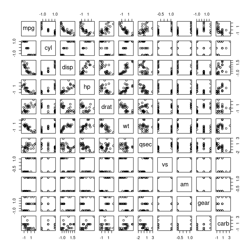
round(cor(dt),2)| mpg | cyl | disp | hp | drat | wt | qsec | vs | am | gear | carb | |
|---|---|---|---|---|---|---|---|---|---|---|---|
| mpg | 1.00 | -0.85 | -0.85 | -0.78 | 0.68 | -0.87 | 0.42 | 0.66 | 0.60 | 0.48 | -0.55 |
| cyl | -0.85 | 1.00 | 0.90 | 0.83 | -0.70 | 0.78 | -0.59 | -0.81 | -0.52 | -0.49 | 0.53 |
| disp | -0.85 | 0.90 | 1.00 | 0.79 | -0.71 | 0.89 | -0.43 | -0.71 | -0.59 | -0.56 | 0.39 |
| hp | -0.78 | 0.83 | 0.79 | 1.00 | -0.45 | 0.66 | -0.71 | -0.72 | -0.24 | -0.13 | 0.75 |
| drat | 0.68 | -0.70 | -0.71 | -0.45 | 1.00 | -0.71 | 0.09 | 0.44 | 0.71 | 0.70 | -0.09 |
| wt | -0.87 | 0.78 | 0.89 | 0.66 | -0.71 | 1.00 | -0.17 | -0.55 | -0.69 | -0.58 | 0.43 |
| qsec | 0.42 | -0.59 | -0.43 | -0.71 | 0.09 | -0.17 | 1.00 | 0.74 | -0.23 | -0.21 | -0.66 |
| vs | 0.66 | -0.81 | -0.71 | -0.72 | 0.44 | -0.55 | 0.74 | 1.00 | 0.17 | 0.21 | -0.57 |
| am | 0.60 | -0.52 | -0.59 | -0.24 | 0.71 | -0.69 | -0.23 | 0.17 | 1.00 | 0.79 | 0.06 |
| gear | 0.48 | -0.49 | -0.56 | -0.13 | 0.70 | -0.58 | -0.21 | 0.21 | 0.79 | 1.00 | 0.27 |
| carb | -0.55 | 0.53 | 0.39 | 0.75 | -0.09 | 0.43 | -0.66 | -0.57 | 0.06 | 0.27 | 1.00 |
- 전반적으로 corr이 높음, 다중공산성 생각!
cars_fit_lm <- lm(mpg~., dt)
summary(cars_fit_lm)
Call:
lm(formula = mpg ~ ., data = dt)

Residuals:
     Min       1Q   Median       3Q      Max
-0.57254 -0.26620 -0.01985  0.20230  0.76773

Coefficients:
              Estimate Std. Error t value Pr(>|t|)
(Intercept) -1.613e-17  7.773e-02   0.000   1.0000
cyl         -3.302e-02  3.097e-01  -0.107   0.9161
disp         2.742e-01  3.672e-01   0.747   0.4635
hp          -2.444e-01  2.476e-01  -0.987   0.3350
drat         6.983e-02  1.451e-01   0.481   0.6353
wt          -6.032e-01  3.076e-01  -1.961   0.0633 .
qsec         2.434e-01  2.167e-01   1.123   0.2739
vs           2.657e-02  1.760e-01   0.151   0.8814
am           2.087e-01  1.703e-01   1.225   0.2340
gear         8.023e-02  1.828e-01   0.439   0.6652
carb        -5.344e-02  2.221e-01  -0.241   0.8122
---
Signif. codes:  0 ‘***’ 0.001 ‘**’ 0.01 ‘*’ 0.05 ‘.’ 0.1 ‘ ’ 1

Residual standard error: 0.4397 on 21 degrees of freedom
Multiple R-squared:  0.869, Adjusted R-squared:  0.8066
F-statistic: 13.93 on 10 and 21 DF,  p-value: 3.793e-07
모형은 유의하지만 모든 회귀계수가 유의하지 않게 나옴.
p-value: \(H_0:\beta_1=\dots=\beta_10=0\) 한개라도 0이 아닌 회귀계수가 존재한다는 뜻이지만 회귀계수 보면 엥 없음.
vif(cars_fit_lm)- cyl
- 15.3738334034422
- disp
- 21.6202410289588
- hp
- 9.83203684435904
- drat
- 3.37462000831475
- wt
- 15.164886963987
- qsec
- 7.5279582252911
- vs
- 4.96587346648471
- am
- 4.64848745550015
- gear
- 5.35745210594066
- carb
- 7.90874675118444
- cyl, disp, wt 가 vif값이 높게 나옴.
능형회귀 (Ridge Regression)
lm.ridge 함수 이용
rfit <- lm.ridge(mpg~., dt, lambda=seq(0.01,20,0.1))\(\hat\beta(\lambda) = (X^TX+\lambda I_p)^{-1} X^Ty\)
람다 범위는 0.01~0.1 범위에서 정해줘.
select(rfit) modified HKB estimator is 2.58585
modified L-W estimator is 1.837435
smallest value of GCV at 14.91 람다 값 몇개 추전해주는 함수.
smallest value of GCV이것을 많이 씀MSE를 가장 작게 하는 \(\lambda\)값을 찾아줘! GCV
round(rfit$coef[,rfit$lam=='0.21'],3)- cyl
- -0.032
- disp
- 0.185
- hp
- -0.211
- drat
- 0.074
- wt
- -0.52
- qsec
- 0.207
- vs
- 0.027
- am
- 0.201
- gear
- 0.082
- carb
- -0.093
- 람다=0.21일 때
round(rfit$coef[,rfit$lam=='3.21'],3)- cyl
- -0.078
- disp
- -0.049
- hp
- -0.144
- drat
- 0.086
- wt
- -0.291
- qsec
- 0.085
- vs
- 0.041
- am
- 0.169
- gear
- 0.075
- carb
- -0.175
round(rfit$coef[,rfit$lam=='14.91'],3)- cyl
- -0.109
- disp
- -0.107
- hp
- -0.13
- drat
- 0.092
- wt
- -0.197
- qsec
- 0.047
- vs
- 0.063
- am
- 0.132
- gear
- 0.066
- carb
- -0.144
\(\hat \beta(14.91)\)
\(\hat \beta^{Ridge}(\lambda) = argmin\{\sum \epsilon_i^2\}\)
\(\sum \beta_j^2 \leq t\)
\(min\{\sum \epsilon_i^2 + \lambda \sum \beta_j^2 \}\)
- 람다의 값이 커질 때, \(\sum \hat \beta_j^2\)의 계수 값은 작아진다.
sum(rfit$coef[,rfit$lam=='0.21']^2)
0.45567046636623
- 람다=0.21 일 때 \(\sum \hat \beta_j^2\)의 계수값
sum(rfit$coef[,rfit$lam=='3.21']^2)
0.195026451544005
- 람다=3.21 일 때 \(\sum \hat \beta_j^2\)의 계수값
sum(rfit$coef[,rfit$lam=='14.91']^2)
0.135989355255867
- 람다=14.91 일 때 \(\sum \hat \beta_j^2\)의 계수값
matplot(rfit$lambda, t(rfit$coef), type='l',
        xlab=expression(lambda),
        ylab=expression(bold(beta)(lambda)), lwd=2)
abline(h=0, col="grey", lty=2)
abline(v=14.91, col="black", lty=2)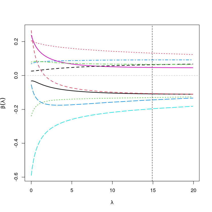
glmnet 함수 이용
매트릭스를 만들어 줘야 함!
그런데 X하뭇에서 1열은 필요 없음(1 1 1 1 .. 이렇게 되어있는) 그래서 아래와 같이 [,-1]로 X(상수항 빠짐)를 가져옴
X <- model.matrix(mpg~., dt)[,-1]
y <- dt$mpg- X <- as.matrix(dt[,-1]) 해도 같은 결과 나올듯
head(X)| cyl | disp | hp | drat | wt | qsec | vs | am | gear | carb | |
|---|---|---|---|---|---|---|---|---|---|---|
| Mazda RX4 | -0.1049878 | -0.57061982 | -0.5350928 | 0.5675137 | -0.610399567 | -0.7771651 | -0.8680278 | 1.1899014 | 0.4235542 | 0.7352031 |
| Mazda RX4 Wag | -0.1049878 | -0.57061982 | -0.5350928 | 0.5675137 | -0.349785269 | -0.4637808 | -0.8680278 | 1.1899014 | 0.4235542 | 0.7352031 |
| Datsun 710 | -1.2248578 | -0.99018209 | -0.7830405 | 0.4739996 | -0.917004624 | 0.4260068 | 1.1160357 | 1.1899014 | 0.4235542 | -1.1221521 |
| Hornet 4 Drive | -0.1049878 | 0.22009369 | -0.5350928 | -0.9661175 | -0.002299538 | 0.8904872 | 1.1160357 | -0.8141431 | -0.9318192 | -1.1221521 |
| Hornet Sportabout | 1.0148821 | 1.04308123 | 0.4129422 | -0.8351978 | 0.227654255 | -0.4637808 | -0.8680278 | -0.8141431 | -0.9318192 | -0.5030337 |
| Valiant | -0.1049878 | -0.04616698 | -0.6080186 | -1.5646078 | 0.248094592 | 1.3269868 | 1.1160357 | -0.8141431 | -0.9318192 | -1.1221521 |
head(y) #mpg- 0.150884824647657
- 0.150884824647657
- 0.449543446630647
- 0.217253407310543
- -0.230734525663942
- -0.330287399658272
Lidge
ridge.fit<-glmnet(X,y,alpha=0, lambda=seq(0.01,20,0.1)) ##ridge : alpha=0
plot(ridge.fit, label=TRUE)
abline(h=0, col="grey", lty=2)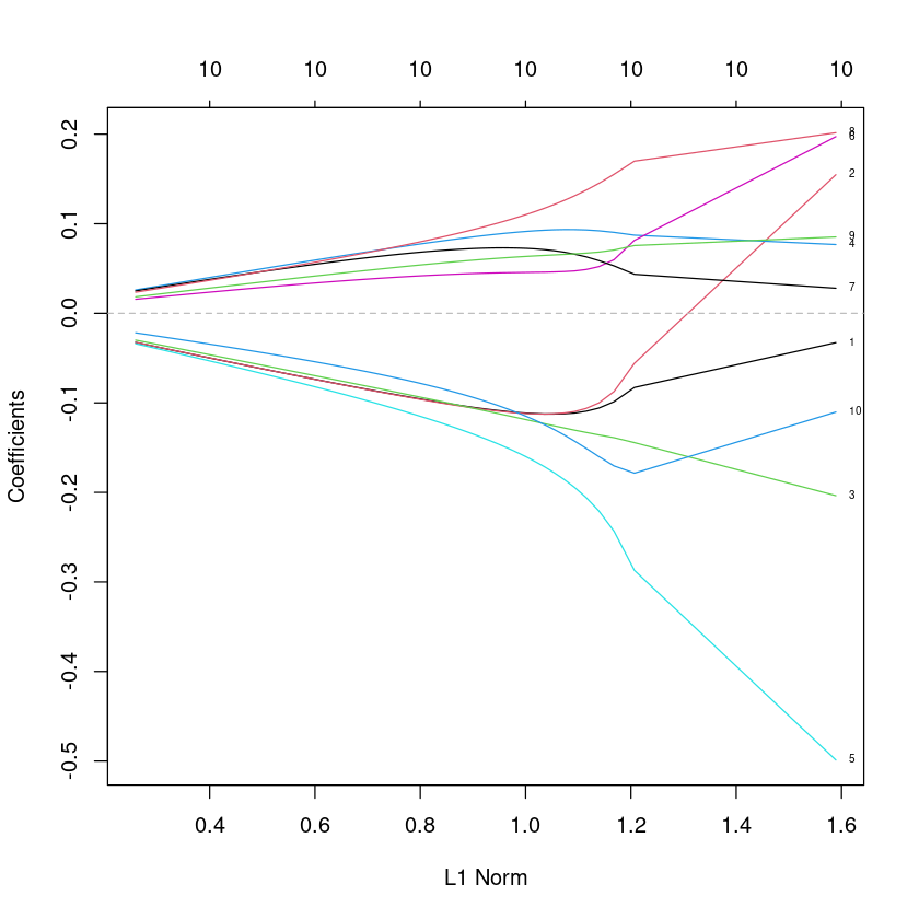
- 위 plot에서 xlabel이 L1 Norm아님. \(\sum |\beta_j|\)
- 최소제곱추정량을 구할 때의 제약 조건
릿지 \(\sum \beta_j^2 \leq t\) : \(L_2\)-norm
라쏘 \(\sum |\beta_j| \leq t\) : \(L_1\)-norm
그런데 릿지 라쏘의 중간 정도를 제약 조건을 주면 어쩔까? 싶어서 나온…
\[(1-\alpha)\sum \beta_j^2 + \alpha \sum|\beta_j| \leq t\]
- \(\alpha=0\)이라면 뒷 부분으 날라가니까 \(Ridge\)를 쓴다는 것이고, \(\alpha=1\)이라면 앞부분 날라가서 \(Rasso\)를 쓴다는 뜻
- 람다를 크게하면서 MSE값이 작아지려면?
Loocv
cv.fit<-cv.glmnet(X,y,alpha=0,nfolds=length(y))Warning message:
“Option grouped=FALSE enforced in cv.glmnet, since < 3 observations per fold”cv.fit
Call:  cv.glmnet(x = X, y = y, nfolds = length(y), alpha = 0)

Measure: Mean-Squared Error

    Lambda Index Measure      SE Nonzero
min 0.4558    82  0.2020 0.05006      10
1se 1.8399    67  0.2465 0.07432      10
cross validatiom
MSE기준으로 람다가 0.4558일때 MSE가 가장 작음
plot(cv.fit)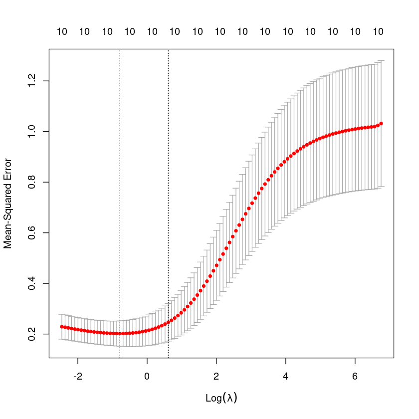
가장 작아지는 값 log(0.4558)=-0.7857
log(1.8399)=0.6097
cv.fit<-cv.glmnet(X,y,alpha=0,nfolds=10)
cv.fit
Call:  cv.glmnet(x = X, y = y, nfolds = 10, alpha = 0)

Measure: Mean-Squared Error

    Lambda Index Measure      SE Nonzero
min 0.5002    81  0.2169 0.05967      10
1se 2.2161 65 0.2764 0.10178 10plot(cv.fit)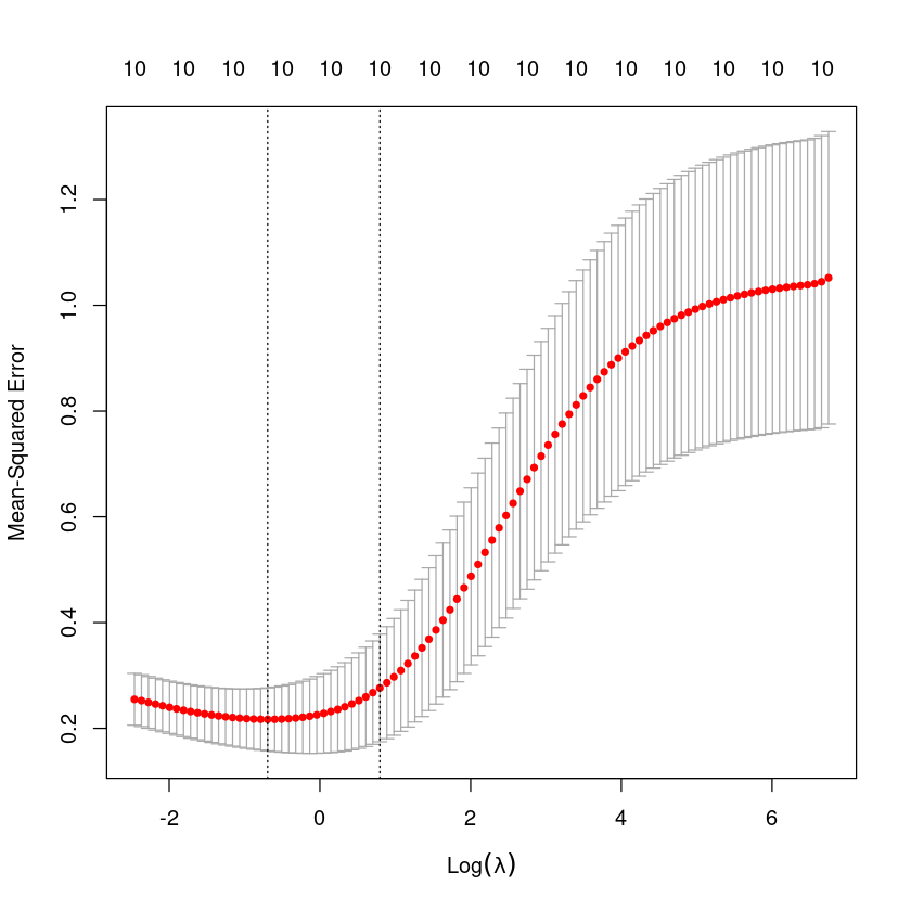
lam<-cv.fit$lambda.min;lam
0.500186412336802
log(lam)
-0.692774425368192
- \(\hat \beta(\lambda)\)의 추정량
predict(ridge.fit,type="coefficients",s=lam)11 x 1 sparse Matrix of class "dgCMatrix"
s1
(Intercept) 8.350503e-17
cyl -1.111861e-01
disp -1.093455e-01
hp -1.307062e-01
drat 9.342524e-02
wt -1.954335e-01
qsec 4.746741e-02
vs 6.573455e-02
am 1.317846e-01
gear 6.643998e-02
carb -1.434548e-01옵션 타입을 ‘coefficients’ 주어야 \(\hat \beta(\lambda)\)의 추정량을 구할 수 있다.
옵션 타입을 ’response’를 쓰게 되면 \(\hat y\)값을 구할 수 있다.
predict(ridge.fit,type="response",s=lam)ERROR: Error in predict.glmnet(ridge.fit, type = "response", s = lam): You need to supply a value for 'newx's1: \(\hat \beta (0.5)\)\(\hat y = X \hat \beta (0.5)\)
Lasso
lasso.fit<-glmnet(X,y,alpha=1, lambda=seq(0.01,20,0.1)) ##lasso : alpha=1
plot(lasso.fit, label=TRUE)
Warning message in regularize.values(x, y, ties, missing(ties), na.rm = na.rm):
“collapsing to unique 'x' values”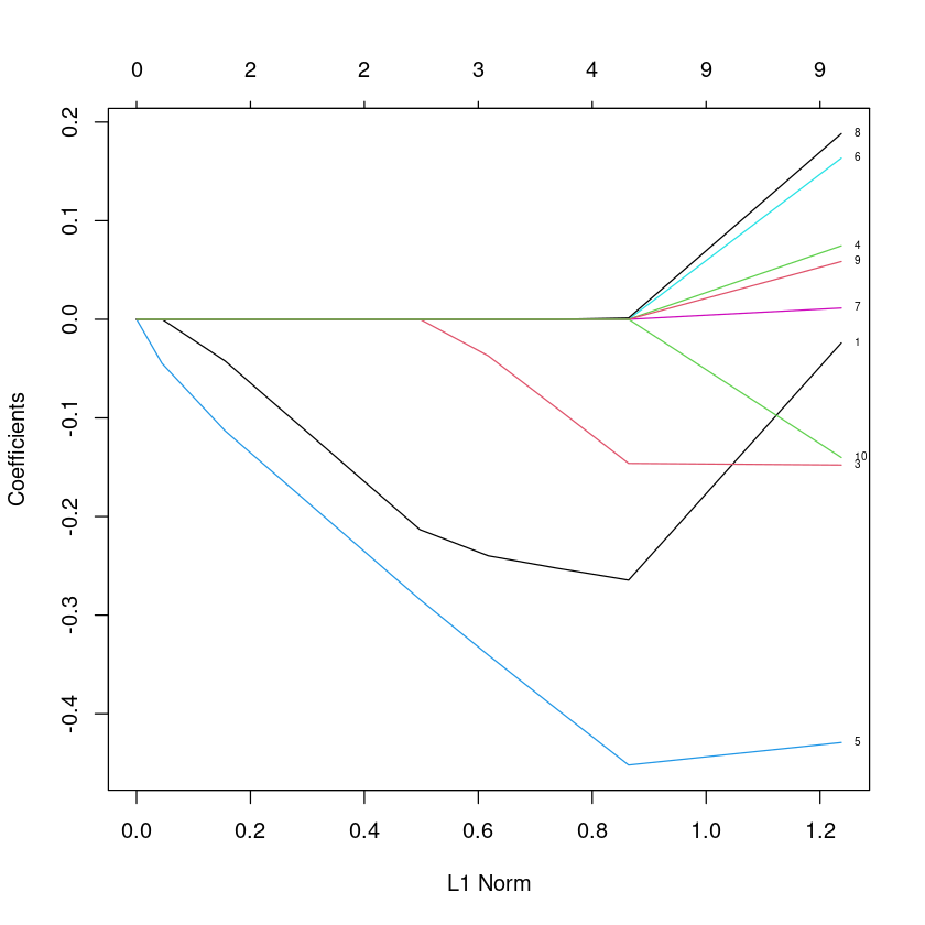
8번 보면 가다가 0이 됨. (릿지는 0으로 수렴하긴 했지만 아예 0은 아니였는데..)
제약조건을 걸면 변수를 포기해버림 (9개 -> 9개 -> 4개 -> 3개 -> 2개 ->)
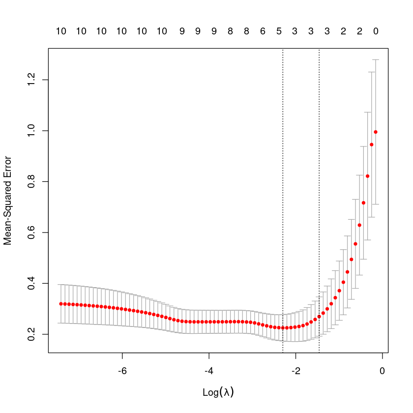
cv.lasso.fit<-cv.glmnet(X,y,alpha=1,nfolds=10)
cv.lasso.fit
Call:  cv.glmnet(x = X, y = y, nfolds = 10, alpha = 1)

Measure: Mean-Squared Error

    Lambda Index Measure      SE Nonzero
min 0.1005    24  0.2252 0.05178       5
1se 0.2322 15 0.2697 0.07727 3plot(cv.lasso.fit)