library(tidyverse)1번
‘dt.csv’ 데이터를 이용하여 회귀모형을 적합하려고 한다. 이는 매장별 유아 카시트 판매액(Sales)를 예측하기 위한 데이터 이다. 다음 물음에 답하여라. (R을 이용하여 풀이)(검정에서는 유의수준 \(α = 0.05\) 사용)
(1)
이 데이터의 산점도 행렬을 그리시오.
dt <- read_csv('dt.csv')
head(dt)
Rows: 400 Columns: 8
── Column specification ────────────────────────────────────────────────────────
Delimiter: ","
dbl (8): Sales, CompPrice, Income, Advertising, Population, Price, Age, Educ...
ℹ Use `spec()` to retrieve the full column specification for this data.
ℹ Specify the column types or set `show_col_types = FALSE` to quiet this message.| Sales | CompPrice | Income | Advertising | Population | Price | Age | Education |
|---|---|---|---|---|---|---|---|
| <dbl> | <dbl> | <dbl> | <dbl> | <dbl> | <dbl> | <dbl> | <dbl> |
| 9.50 | 138 | 73 | 11 | 276 | 120 | 42 | 17 |
| 11.22 | 111 | 48 | 16 | 260 | 83 | 65 | 10 |
| 10.06 | 113 | 35 | 10 | 269 | 80 | 59 | 12 |
| 7.40 | 117 | 100 | 4 | 466 | 97 | 55 | 14 |
| 4.15 | 141 | 64 | 3 | 340 | 128 | 38 | 13 |
| 10.81 | 124 | 113 | 13 | 501 | 72 | 78 | 16 |
pairs(dt, pch=16, col='darkorange')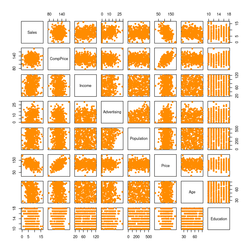
- 선형관계가 있어보이는 데이터는, “sales와 price”,“compprice와 porice”,
pairs(dt[,which(names(dt) %in%
                      c('Sales', 'CompPrice', 'Price'))],
      pch=16, col='darkorange')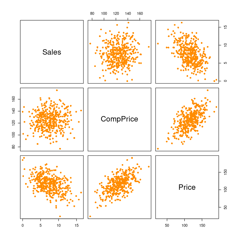
cor(dt[,which(names(dt) %in%
c('Sales', 'CompPrice', 'Price'))])| Sales | CompPrice | Price | |
|---|---|---|---|
| Sales | 1.00000000 | 0.06407873 | -0.4449507 |
| CompPrice | 0.06407873 | 1.00000000 | 0.5848478 |
| Price | -0.44495073 | 0.58484777 | 1.0000000 |
- 2,3번 문제에서 축소모형 하니까.. 1번 문제에서는 걍 전체로 돌리자
(2)
Sales를 예측하기 위한 중회귀분석을 하려고 한다. 이를 위한 모형을 설정하시오.
fit_dt<-lm(Sales~., data=dt)
summary(fit_dt)
Call:
lm(formula = Sales ~ ., data = dt)

Residuals:
    Min      1Q  Median      3Q     Max
-5.0598 -1.3515 -0.1739  1.1331  4.8304

Coefficients:
              Estimate Std. Error t value Pr(>|t|)
(Intercept)  7.7076934  1.1176260   6.896 2.15e-11 ***
CompPrice    0.0939149  0.0078395  11.980  < 2e-16 ***
Income       0.0128717  0.0034757   3.703 0.000243 ***
Advertising  0.1308637  0.0151219   8.654  < 2e-16 ***
Population  -0.0001239  0.0006877  -0.180 0.857092
Price       -0.0925226  0.0050521 -18.314  < 2e-16 ***
Age         -0.0449743  0.0060083  -7.485 4.75e-13 ***
Education   -0.0399844  0.0371257  -1.077 0.282142
---
Signif. codes:  0 ‘***’ 0.001 ‘**’ 0.01 ‘*’ 0.05 ‘.’ 0.1 ‘ ’ 1

Residual standard error: 1.929 on 392 degrees of freedom
Multiple R-squared:  0.5417,    Adjusted R-squared:  0.5335
F-statistic: 66.18 on 7 and 392 DF,  p-value: < 2.2e-16
\(\widehat {Sales} = 7.7076934 + 0.0939149 \widehat {CompPrice} + 0.012871 \widehat {Income} +0.1308637 \widehat {Advertising} -0.0001239 \widehat {Population} -0.0925226 \widehat {Price} -0.0449743 \widehat {Age} -0.0399844 \widehat {Education}\)
fit__<-lm(Sales~CompPrice+Price, data=dt)
summary(fit__)
Call:
lm(formula = Sales ~ CompPrice + Price, data = dt)

Residuals:
    Min      1Q  Median      3Q     Max
-5.5285 -1.6207 -0.2404  1.5269  6.2437

Coefficients:
             Estimate Std. Error t value Pr(>|t|)
(Intercept)  6.278692   0.932774   6.731 5.91e-11 ***
CompPrice    0.090777   0.009132   9.941  < 2e-16 ***
Price       -0.087458   0.005914 -14.788  < 2e-16 ***
---
Signif. codes:  0 ‘***’ 0.001 ‘**’ 0.01 ‘*’ 0.05 ‘.’ 0.1 ‘ ’ 1

Residual standard error: 2.269 on 397 degrees of freedom
Multiple R-squared:  0.3578,    Adjusted R-squared:  0.3546
F-statistic: 110.6 on 2 and 397 DF,  p-value: < 2.2e-16
\(\widehat {Sales} = 6.278692 + 0.090777 \widehat {CompPrice} -0.087458 \widehat {Price}\)
(3)
최소제곱법의 의한 회귀직선을 적합시키시키고, 모형 적합 결과를 설명하시오.
(4)
회귀직선의 유의성 검정을 위한 가설을 설정하고, 분산분석표를 이용하여 가설 검정을 수행하시오.
\(H_0:\beta_0=\dots=\beta_7=0\) vs. \(H_1:not H_0\)
anova(fit_dt)| Df | Sum Sq | Mean Sq | F value | Pr(>F) | |
|---|---|---|---|---|---|
| <int> | <dbl> | <dbl> | <dbl> | <dbl> | |
| CompPrice | 1 | 13.0666859 | 13.0666859 | 3.5117751 | 6.167778e-02 |
| Income | 1 | 79.0733616 | 79.0733616 | 21.2515906 | 5.458487e-06 |
| Advertising | 1 | 219.3512681 | 219.3512681 | 58.9523862 | 1.300900e-13 |
| Population | 1 | 0.3824026 | 0.3824026 | 0.1027737 | 7.486970e-01 |
| Price | 1 | 1198.8668836 | 1198.8668836 | 322.2049460 | 5.144277e-53 |
| Age | 1 | 208.6564283 | 208.6564283 | 56.0780635 | 4.652175e-13 |
| Education | 1 | 4.3158913 | 4.3158913 | 1.1599299 | 2.821424e-01 |
| Residuals | 392 | 1458.5617763 | 3.7208209 | NA | NA |
null_model <- lm(Sales~1, data=dt)
fit_dt <- lm(Sales~., data=dt)

anova(null_model, fit_dt) | Res.Df | RSS | Df | Sum of Sq | F | Pr(>F) | |
|---|---|---|---|---|---|---|
| <dbl> | <dbl> | <dbl> | <dbl> | <dbl> | <dbl> | |
| 1 | 399 | 3182.275 | NA | NA | NA | NA |
| 2 | 392 | 1458.562 | 7 | 1723.713 | 66.18021 | 1.413772e-62 |
- 회귀직선은 유의하다.
(1723.713/7)/(1458.562/392)
66.1802021443038
(5)
오차의 분산에 대한 추정량을 구하시오.
matrix
n = nrow(dt)
X = cbind(rep(1,n), dt$CompPrice, dt$Income, dt$Advertising, dt$Population, dt$Price, dt$Age, dt$Education)
y = dt$Sales
beta_hat = solve(t(X)%*%X) %*% t(X) %*% y # t(X): X^T를 의미함
beta_hat
coef(fit_dt)| 7.7076934384 |
| 0.0939149066 |
| 0.0128717129 |
| 0.1308636707 |
| -0.0001239252 |
| -0.0925226099 |
| -0.0449743402 |
| -0.0399844437 |
- (Intercept)
- 7.70769343844283
- CompPrice
- 0.0939149066067561
- Income
- 0.0128717128971186
- Advertising
- 0.130863670692396
- Population
- -0.000123925156795604
- Price
- -0.0925226098938757
- Age
- -0.0449743402082049
- Education
- -0.0399844437382063
y_hat = X %*% beta_hat
y_hat[1:5]
fitted(fit_dt)[1:5]- 9.3415116064463
- 9.80913530905876
- 9.51078048749865
- 8.44055027735586
- 8.05222459125309
- 1
- 9.34151160644671
- 2
- 9.80913530905893
- 3
- 9.51078048749877
- 4
- 8.44055027735589
- 5
- 8.05222459125317
sse <- sum((y - y_hat)^2) ##SSE
sqrt(sse/(n-7-1)) ##RMSE
summary(fit_dt)$sigma
1.92894293798154
1.92894293798154
mse <- sse/(n-7-1)
mse
3.72082085798886
(6)
결정계수와 수정된 결정계수를 구하시오.
summary(fit_dt)
Call:
lm(formula = Sales ~ ., data = dt)

Residuals:
    Min      1Q  Median      3Q     Max
-5.0598 -1.3515 -0.1739  1.1331  4.8304

Coefficients:
              Estimate Std. Error t value Pr(>|t|)
(Intercept)  7.7076934  1.1176260   6.896 2.15e-11 ***
CompPrice    0.0939149  0.0078395  11.980  < 2e-16 ***
Income       0.0128717  0.0034757   3.703 0.000243 ***
Advertising  0.1308637  0.0151219   8.654  < 2e-16 ***
Population  -0.0001239  0.0006877  -0.180 0.857092
Price       -0.0925226  0.0050521 -18.314  < 2e-16 ***
Age         -0.0449743  0.0060083  -7.485 4.75e-13 ***
Education   -0.0399844  0.0371257  -1.077 0.282142
---
Signif. codes:  0 ‘***’ 0.001 ‘**’ 0.01 ‘*’ 0.05 ‘.’ 0.1 ‘ ’ 1

Residual standard error: 1.929 on 392 degrees of freedom
Multiple R-squared:  0.5417,    Adjusted R-squared:  0.5335
F-statistic: 66.18 on 7 and 392 DF, p-value: < 2.2e-16- \(R^2:0.5417, R^2_{adj}: 0.5335\)
(7)
개별 회귀계수의 유의성검정을 수행하시오.
summary(fit_dt)$coef| Estimate | Std. Error | t value | Pr(>|t|) | |
|---|---|---|---|---|
| (Intercept) | 7.7076934384 | 1.1176259965 | 6.8964873 | 2.145154e-11 |
| CompPrice | 0.0939149066 | 0.0078395225 | 11.9796718 | 2.153866e-28 |
| Income | 0.0128717129 | 0.0034756701 | 3.7033759 | 2.432641e-04 |
| Advertising | 0.1308636707 | 0.0151219066 | 8.6539134 | 1.302560e-16 |
| Population | -0.0001239252 | 0.0006877272 | -0.1801952 | 8.570924e-01 |
| Price | -0.0925226099 | 0.0050520870 | -18.3137403 | 1.409811e-54 |
| Age | -0.0449743402 | 0.0060082977 | -7.4853715 | 4.751078e-13 |
| Education | -0.0399844437 | 0.0371257460 | -1.0770004 | 2.821424e-01 |
(8)
회귀계수에 대한 90% 신뢰구간을 구하시오.
confint(fit_dt, level = 0.90)| 5 % | 95 % | |
|---|---|---|
| (Intercept) | 5.865007519 | 9.550379358 |
| CompPrice | 0.080989493 | 0.106840320 |
| Income | 0.007141202 | 0.018602224 |
| Advertising | 0.105931426 | 0.155795915 |
| Population | -0.001257815 | 0.001009965 |
| Price | -0.100852239 | -0.084192981 |
| Age | -0.054880521 | -0.035068159 |
| Education | -0.101195519 | 0.021226632 |
(9)
CompPrice = 100, Income = 70, Advertising = 20, Population = 300, Price = 80, Education = 12인 지역에 위치한 매장의 평균 판매액을 예측하고, 95% 신뢰구간을 구하시오.
new_dt <- data.frame(CompPrice=100, Income=70, Advertising=20, Population=300, Price=80, Age=53, Education=12)predict(fit_dt,
newdata = new_dt,
interval = c("confidence"),
level = 0.95) ##평균반응| fit | lwr | upr | |
|---|---|---|---|
| 1 | 10.31504 | 9.746147 | 10.88393 |
- 문제에서 Age에 대한 값이 명시되지 않아서.. 일단 age는 평균 값 넣어서 계산함
(10)
위 매장에 대하여 개별 판매액 예측하고, 95% 신뢰구간을 구하시오.
predict(fit_dt, newdata = new_dt,
        interval = c("prediction"),
level = 0.95) ## 개별 y| fit | lwr | upr | |
|---|---|---|---|
| 1 | 10.31504 | 6.480238 | 14.14984 |
(11)
잔차에 대한 산점도를 그리고, 결과를 설명하여라.
yhat <- fitted(fit_dt)
res <- resid(fit_dt)plot(res ~ yhat,pch=16, ylab = 'Residual')
abline(h=0, lty=2, col='grey')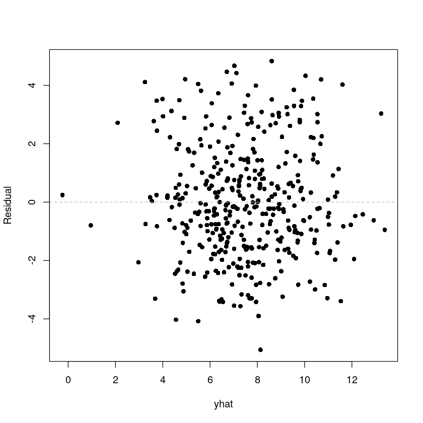
선형성은 없어보이고, 등분산성이 있어보인다.
(12)
잔차에 대한 등분산성 검정을 수행하여라.
\(H_0\):등분산 VS. \(H_1\):이분산
library(lmtest)Loading required package: zoo
Attaching package: ‘zoo’
The following objects are masked from ‘package:base’:
as.Date, as.Date.numeric
bptest(fit_dt)
    studentized Breusch-Pagan test

data:  fit_dt
BP = 1.1751, df = 7, p-value = 0.9915- p-valeur가 커서 \(H_0\)를 채택한다. 즉 등분산성이다.
(13)
잔차에 대한 히스토그램, QQ plot을 그리고, 정규성 검정을 수행하여라.
par(mfrow=c(1,2))
qqnorm(res, pch=16)
qqline(res, col = 2)

hist(res)
par(mfrow=c(1,1))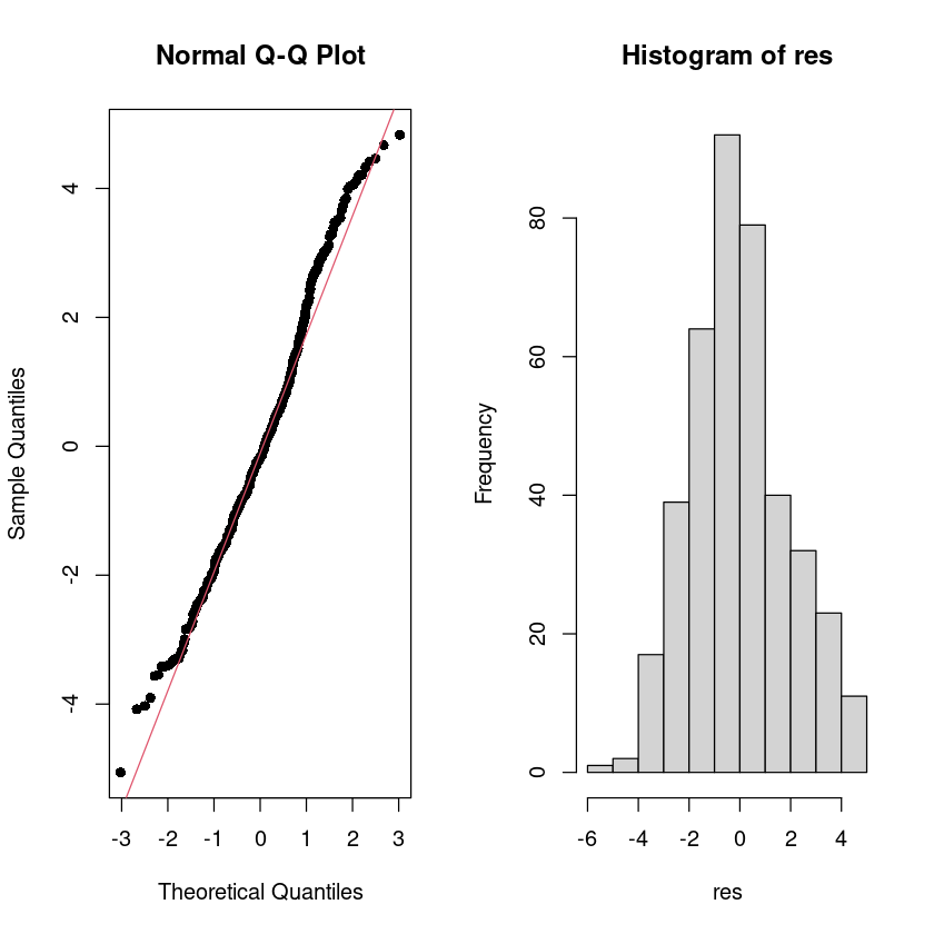
- 정규성을 만족해 보인다.
## H0 : normal distribution  vs. H1 : not H0
shapiro.test(res)
    Shapiro-Wilk normality test

data:  res
W = 0.98602, p-value = 0.0006715
(14)
잔차에 대한 독립성 검정을 수행하시오.
\(H_0\):uncorrelated
dwtest(fit_dt, alternative = "two.sided")
    Durbin-Watson test

data:  fit_dt
DW = 1.9694, p-value = 0.7622
alternative hypothesis: true autocorrelation is not 0- 독립이다.
2번
위 데이터에 대하여 다음 물음에 답하여라. (R을 이용하여 풀이)(검정에서는 유의수준 \(α = 0.05\) 사용)
(1)
위에서 적합한 모형에서 개별 회귀계수의 유의성 검정 결과 유의하지 않은 변수는 무엇인가?
Population, Education은 유의하지 않은 변수이다.
(2)
위에서 유의하지 않았던 변수를 제외한 모형을 축소모형(Reduced Model)으로 하는 부분 F검정을 수행하여라. 검정에 필요한 가설을 설정하고, 검정 결과를 설명하시오.
reduced_model<-lm(Sales~.-Population-Education, data=dt)anova(reduced_model, fit_dt)| Res.Df | RSS | Df | Sum of Sq | F | Pr(>F) | |
|---|---|---|---|---|---|---|
| <dbl> | <dbl> | <dbl> | <dbl> | <dbl> | <dbl> | |
| 1 | 394 | 1462.897 | NA | NA | NA | NA |
| 2 | 392 | 1458.562 | 2 | 4.335087 | 0.5825445 | 0.5589583 |
(3)
1번에서 설정한 모형과, 축소모형 중 어느 모형이 이 데이터에 대한 설명을 잘 하고 있는지를 비교하시오.
summary(reduced_model)
summary(fit_dt)
Call:
lm(formula = Sales ~ . - Population - Education, data = dt)

Residuals:
    Min      1Q  Median      3Q     Max
-4.9071 -1.3081 -0.1892  1.1495  4.6980

Coefficients:
             Estimate Std. Error t value Pr(>|t|)
(Intercept)  7.109190   0.943940   7.531 3.46e-13 ***
CompPrice    0.093904   0.007792  12.051  < 2e-16 ***
Income       0.013092   0.003465   3.779 0.000182 ***
Advertising  0.130611   0.014572   8.963  < 2e-16 ***
Price       -0.092543   0.005044 -18.347  < 2e-16 ***
Age         -0.044971   0.005994  -7.503 4.20e-13 ***
---
Signif. codes:  0 ‘***’ 0.001 ‘**’ 0.01 ‘*’ 0.05 ‘.’ 0.1 ‘ ’ 1

Residual standard error: 1.927 on 394 degrees of freedom
Multiple R-squared:  0.5403,    Adjusted R-squared:  0.5345
F-statistic: 92.62 on 5 and 394 DF,  p-value: < 2.2e-16
Call:
lm(formula = Sales ~ ., data = dt)

Residuals:
    Min      1Q  Median      3Q     Max
-5.0598 -1.3515 -0.1739  1.1331  4.8304

Coefficients:
              Estimate Std. Error t value Pr(>|t|)
(Intercept)  7.7076934  1.1176260   6.896 2.15e-11 ***
CompPrice    0.0939149  0.0078395  11.980  < 2e-16 ***
Income       0.0128717  0.0034757   3.703 0.000243 ***
Advertising  0.1308637  0.0151219   8.654  < 2e-16 ***
Population  -0.0001239  0.0006877  -0.180 0.857092
Price       -0.0925226  0.0050521 -18.314  < 2e-16 ***
Age         -0.0449743  0.0060083  -7.485 4.75e-13 ***
Education   -0.0399844  0.0371257  -1.077 0.282142
---
Signif. codes:  0 ‘***’ 0.001 ‘**’ 0.01 ‘*’ 0.05 ‘.’ 0.1 ‘ ’ 1

Residual standard error: 1.929 on 392 degrees of freedom
Multiple R-squared:  0.5417,    Adjusted R-squared:  0.5335
F-statistic: 66.18 on 7 and 392 DF,  p-value: < 2.2e-16
3번
1번에서 설정한 모형에 대하여 아래의 일반 선형 가설검정(General Linear Hypothesis Test)을 수행하시오. (R을 이용하여 풀이)(검정에서는 유의수준 \(α = 0.05\) 사용)(회귀계수는 \(β_i\)로 표현해야 하지만, 각자 설정이 다를 수가 있기 때문에 회귀계수 대신 변수 이름을 사용하겠음. 예 \(β_1 =CompPrice\))
(1)
\(H_0 : CompPrice=Income\) vs. \(H_1 : not H_0\)
install.packages("car")Installing package into ‘/home/coco/R/x86_64-pc-linux-gnu-library/4.2’
(as ‘lib’ is unspecified)
linearHypothesis(dt_fit, c(0,1,-1,0,0,0,0,0),0)(2)
\(H_0 : CompPrice=-Price\) vs. \(H_1 : not H_0\)
linearHypothesis(fit_dt, c(0,1,0,0,0,1,0,0),0)(3)
\(H_0\)를 기각할 수 있는 제약조건을 만들어 보시오.(단 2개 이상의 변수 사용)