library(ggplot2)

1번

중학교 2학년 학생 중에서 15명을 임의로 추출하여 각 학생의 약력(kg), 신장(cm), 체중(kg)과 원반던지기에서 던진 거리(m)를 측정하여 다음의 데이터를 얻었다. 다음 물음에 답하여라. (R을 이용하여 풀이)(검정에서는 유의수준 α = 0.05 사용)

학생번호	x1(약력)	x2(신장)	x3(체중)	y(원반던지기 거리)
1	28	146	34	22
2	47	169	57	36
3	39	160	38	24
4	25	156	28	22
5	34	161	37	27
6	29	168	50	29
7	38	154	54	26
8	23	153	40	23
9	52	160	62	31
10	37	152	39	25
11	35	155	46	23
12	39	154	54	27
13	38	157	57	31
14	32	162	53	25
15	25	142	32	23

dt <- data.frame(x1 = c(28,47,39,25,34,29,38,23,52,37,35,39,38,32,25),
                 x2 = c(146,169,160,156,161,168,154,153,160,152,155,154,157,162,142),
                 x3 = c(34,57,38,28,37,50,54,40,62,39,46,54,57,53,32),
 y = c(22,36,24,22,27,29,26,23,31,25,23,27,31,25,23))

(1)

$x_3$를 설명변수로 하고 $y$를 반응변수로 하여 회귀직선을 적합시키고, 이상치가 있는가, 어떤 것이 영향을 크게 주는 측정값인가를 판정하시오.

model1 <- lm(y~x3,dt)
summary(model1)


Call:
lm(formula = y ~ x3, data = dt)

Residuals:
   Min     1Q Median     3Q    Max 
-3.453 -1.727 -0.042  1.068  6.396 

Coefficients:
            Estimate Std. Error t value Pr(>|t|)    
(Intercept) 13.20655    3.15279   4.189 0.001061 ** 
x3           0.28767    0.06774   4.247 0.000953 ***
---
Signif. codes:  0 ‘***’ 0.001 ‘**’ 0.01 ‘*’ 0.05 ‘.’ 0.1 ‘ ’ 1

Residual standard error: 2.692 on 13 degrees of freedom
Multiple R-squared:  0.5811,    Adjusted R-squared:  0.5489 
F-statistic: 18.04 on 1 and 13 DF,  p-value: 0.0009527

plot(y~x3, dt,pch = 20,cex = 2,col = "darkorange")
abline(model1, col='steelblue', lwd=2)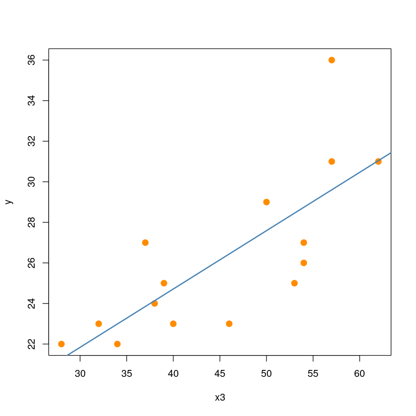

leverage

Hmatrix

X = cbind(rep(1, nrow(dt)), dt$x3)
H = X %*% solve(t(X) %*% X) %*% t(X)
diag(H)

0.148940660082722
0.151852789735798
0.101333670971554
0.258335443572213
0.111336203258209
0.0800624630708194
0.113488646914831
0.0851270363805184
0.241115894319237
0.0925972820123238
0.0668945724656031
0.113488646914831
0.151852789735798
0.103232885962691
0.180341014602853

hatvalues 함수

which.max(hatvalues(model1))
hatvalues(model1)[which.max(hatvalues(model1))]

4: 4

4: 0.258335443572212

2*(1+1)/nrow(dt)

0.266666666666667

$h_{4} < 2\bar h$이므로 leverage포인트로 고려할 점은 없다.

이상치

잔차

residual <- model1$residuals
head(residual)

1: -0.987254157170599
2: 6.39638727103908
3: -0.137925213134126
4: 0.738752426774713
5: 3.14974255085676
6: 1.41006161897527

hist(residual)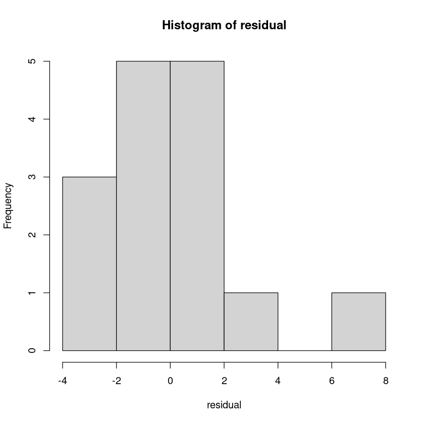

내적표준화된 잔차

s_residual <- rstandard(model1)
head(s_residual)

1: -0.397517137814801
2: 2.57991821095028
3: -0.0540444666750733
4: 0.318641226294653
5: 1.2411181316058
6: 0.546091891647763

hist(s_residual)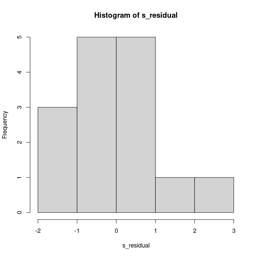

s_residual>2

1: FALSE
2: TRUE
3: FALSE
4: FALSE
5: FALSE
6: FALSE
7: FALSE
8: FALSE
9: FALSE
10: FALSE
11: FALSE
12: FALSE
13: FALSE
14: FALSE
15: FALSE

외적표준화된 잔차

s_residual_i <- rstudent(model1)
head(s_residual_i)

1: -0.384264693530971
2: 3.5482500706297
3: -0.0519300781139025
4: 0.307343141739411
5: 1.27004329309873
6: 0.530791544243437

hist(s_residual_i)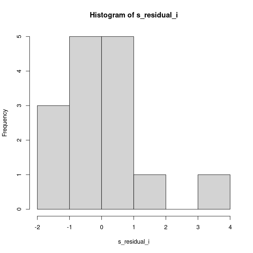

which.max(s_residual_i)
s_residual_i[which.max(s_residual_i)]

2: 2

2: 3.5482500706297

qt(0.975, 15-1-2)

2.17881282966723

$|r_i^*| \geq t_{\alpha/2}(12)$ 이므로 2번째 관측값은 유의수준 0.05에서 이상점이다.

plot(y~x3, dt,pch = 20,cex = 2,col = "darkorange")
abline(model1, col='steelblue', lwd=2)

영향점

influence(model1)

$hat

1: 0.148940660082721
2: 0.151852789735798
3: 0.101333670971554
4: 0.258335443572212
5: 0.111336203258209
6: 0.0800624630708196
7: 0.113488646914831
8: 0.0851270363805183
9: 0.241115894319237
10: 0.0925972820123238
11: 0.0668945724656031
12: 0.113488646914831
13: 0.151852789735798
14: 0.103232885962691
15: 0.180341014602853

$coefficients

A matrix: 15 × 2 of type dbl
	(Intercept)	x3
1	-0.45742205	0.0083719544
2	-2.01160268	0.0553827321
3	-0.04287451	0.0007190015
4	0.56454256	-0.0109721950
5	1.09199851	-0.0188481935
6	-0.10046455	0.0044636533
7	0.55803792	-0.0168311648
8	-0.41549161	0.0064019062
9	0.02268944	-0.0005809430
10	0.15864320	-0.0025647941
11	-0.18216030	-0.0014000365
12	0.35441974	-0.0106897699
13	-0.43915046	0.0120905347
14	0.58437398	-0.0185257601
15	0.32415484	-0.0060864196

$sigma

1: 2.78495746793195
2: 1.95742401077584
3: 2.80172466134264
4: 2.79107580280945
5: 2.63079972749359
6: 2.76971399687302
7: 2.67308548669918
8: 2.75391719372408
9: 2.80200497070363
10: 2.79662725993432
11: 2.60673085648245
12: 2.75075026012413
13: 2.76764179330928
14: 2.59682146853761
15: 2.79575824802225

$wt.res

1: -0.987254157170599
2: 6.39638727103908
3: -0.137925213134126
4: 0.738752426774713
5: 3.14974255085676
6: 1.41006161897527
7: -2.74060943698827
8: -1.71326074111589
9: -0.0419515489153378
10: 0.574407022874991
11: -3.4392673250612
12: -1.74060943698827
13: 1.39638727103908
14: -3.45294167299738
15: 0.588081370811178

influence.measures(model1)

Influence measures of
     lm(formula = y ~ x3, data = dt) :

     dfb.1_   dfb.x3    dffit cov.r   cook.d    hat inf
1  -0.14025  0.11948 -0.16075 1.346 1.38e-02 0.1489    
2  -0.87752  1.12451  1.50138 0.330 5.96e-01 0.1519   *
3  -0.01307  0.01020 -0.01744 1.305 1.65e-04 0.1013    
4   0.17271 -0.15624  0.18139 1.558 1.77e-02 0.2583   *
5   0.35443 -0.28474  0.44954 1.026 9.65e-02 0.1113    
6  -0.03097  0.06405  0.15659 1.218 1.30e-02 0.0801    
7   0.17826 -0.25025 -0.38961 1.096 7.48e-02 0.1135    
8  -0.12883  0.09239 -0.19840 1.197 2.06e-02 0.0851    
9   0.00691 -0.00824 -0.00969 1.546 5.08e-05 0.2411   *
10  0.04844 -0.03645  0.06888 1.283 2.56e-03 0.0926    
11 -0.05967 -0.02135 -0.36571 0.942 6.27e-02 0.0669    
12  0.11002 -0.15445 -0.24046 1.230 3.02e-02 0.1135    
13 -0.13549  0.17362  0.23181 1.317 2.84e-02 0.1519    
14  0.19215 -0.28354 -0.47641 0.965 1.06e-01 0.1032    
15  0.09900 -0.08652  0.10898 1.419 6.40e-03 0.1803

DFFITS

dffits(model1)

1: -0.160752301355561
2: 1.50137779530986
3: -0.0174379982140392
4: 0.181389340447362
5: 0.449539631280775
6: 0.156588296343735
7: -0.389606512891271
8: -0.198401773199523
9: -0.00968760810666192
10: 0.0688785820818028
11: -0.36570800481418
12: -0.240459576775504
13: 0.231812126360193
14: -0.476405218577437
15: 0.108981268211392

which(abs(dffits(model1)) > 2*sqrt(2/(15-2)))

2: 2

Cook’s Distance

cooks.distance(model1)

1: 0.0138272288214354
2: 0.595845162090567
3: 0.000164675041376078
4: 0.0176827743279407
5: 0.0964928567484941
6: 0.0129769331507123
7: 0.0748275851885876
8: 0.0205956959313652
9: 5.08340304142156e-05
10: 0.00255988931413331
11: 0.0626967366405896
12: 0.0301835348837091
13: 0.0283972104088968
14: 0.105589522000774
15: 0.00640451964826487

qf(0.5,2,15-2)

0.731454594627164

which(cooks.distance(model1) >qf(0.5,2,15-2))

없다

COVRATIO

covratio(model1)

1: 1.34567954997946
2: 0.329530512740796
3: 1.30536080523447
4: 1.55778037598378
5: 1.02622098650489
6: 1.2178914729273
7: 1.0964638479128
8: 1.19693328273621
9: 1.54641970673037
10: 1.28341023214919
11: 0.94206589709893
12: 1.22955391198272
13: 1.31702952017448
14: 0.965419184972857
15: 1.41903295690633

which(abs(covratio(model1)-1) > 3*(1+1)/15)

2: 2
4: 4
9: 9
15: 15

summary(influence.measures(model1))

Potentially influential observations of
     lm(formula = y ~ x3, data = dt) :

  dfb.1_ dfb.x3  dffit   cov.r   cook.d hat  
2 -0.88   1.12_*  1.50_*  0.33_*  0.60   0.15
4  0.17  -0.16    0.18    1.56_*  0.02   0.26
9  0.01  -0.01   -0.01    1.55_*  0.00   0.24

영향점은 2번째 관측값이다.

## 2제거 전후
plot(y~x3, dt,pch = 20,
 cex = 2,col = "darkorange",
 main = "2번 제거")
abline(model1, col='steelblue', lwd=2)
abline(lm(y~x3, dt[-2,]), col='red', lwd=2)
text(dt[2,], pos=2, "2")
legend('topright', legend=c("full", "del(2)"),
 col=c('steelblue', 'red'), lty=1, lwd=2)
# high leverage and high influence, not outlier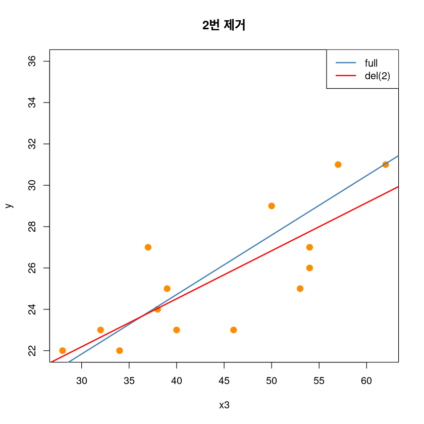

## 4제거 전후
plot(y~x3, dt,pch = 20,
 cex = 2,col = "darkorange",
 main = "4번 제거")
abline(model1, col='steelblue', lwd=2)
abline(lm(y~x3, dt[-4,]), col='red', lwd=2)
text(dt[-4,], pos=2, "2")
legend('topright', legend=c("full", "del(4)"),
 col=c('steelblue', 'red'), lty=1, lwd=2)
# high leverage and high influence, not outlier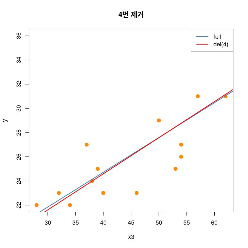

## 9제거 전후
plot(y~x3, dt,pch = 20,
 cex = 2,col = "darkorange",
 main = "9번 제거")
abline(model1, col='steelblue', lwd=2)
abline(lm(y~x3, dt[-9,]), col='red', lwd=2)
legend('topright', legend=c("full", "del(9)"),
 col=c('steelblue', 'red'), lty=1, lwd=2)
# high leverage and high influence, not outlier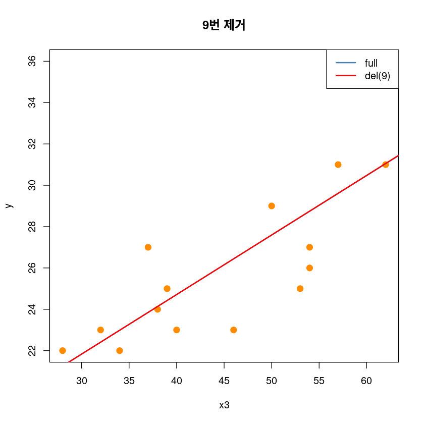

## 4,9제거 전후
plot(y~x3, dt,pch = 20,
 cex = 2,col = "darkorange",
 main = "4,9번 제거")
abline(model1, col='steelblue', lwd=2)
abline(lm(y~x3, dt[-c(4,9),]), col='red', lwd=2)
legend('topright', legend=c("full", "del(4,9)"),
 col=c('steelblue', 'red'), lty=1, lwd=2)
# high leverage and high influence, not outlier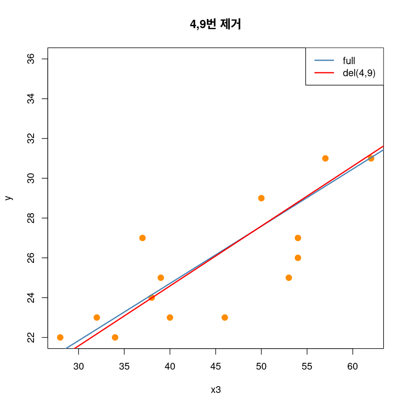

## 2,4,9제거 전후
plot(y~x3, dt,pch = 20,
 cex = 2,col = "darkorange",
 main = "2,4,9번 제거")
abline(model1, col='steelblue', lwd=2)
abline(lm(y~x3, dt[-c(2,4,9),]), col='red', lwd=2)
legend('topright', legend=c("full", "del(2,4,9)"),
 col=c('steelblue', 'red'), lty=1, lwd=2)
# high leverage and high influence, not outlier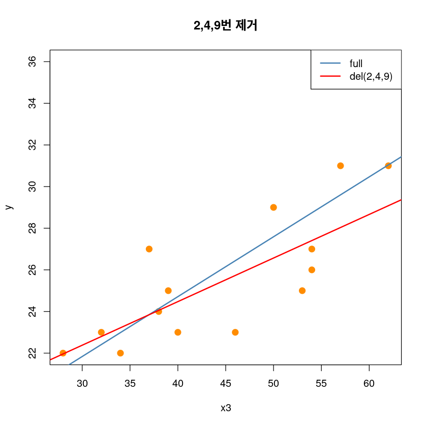

정규성

shapiro.test(model1$residuals)


    Shapiro-Wilk normality test

data:  model1$residuals
W = 0.93332, p-value = 0.3057

회귀진단 그림


par(mfrow = c(2, 2))
plot(model1, pch=16)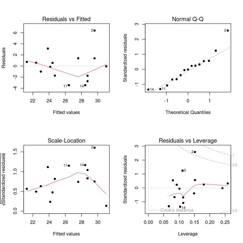

(2)

$x_1, x_2, x_3$ 를 모두 사용하여 $y$에 대한 중회귀모형을 적합시키고, 이상치의 존재유무와 영향을 크게 주는 측정값이 어떤 것인가를 판정하시오.

model2 <- lm(y~x1+x2+x3,dt)
summary(model2)


Call:
lm(formula = y ~ x1 + x2 + x3, data = dt)

Residuals:
    Min      1Q  Median      3Q     Max 
-3.0723 -1.0869 -0.0208  0.9365  3.8745 

Coefficients:
             Estimate Std. Error t value Pr(>|t|)  
(Intercept) -15.78431   14.50462  -1.088   0.2998  
x1            0.15684    0.11331   1.384   0.1937  
x2            0.19620    0.10215   1.921   0.0811 .
x3            0.12948    0.09083   1.425   0.1818  
---
Signif. codes:  0 ‘***’ 0.001 ‘**’ 0.01 ‘*’ 0.05 ‘.’ 0.1 ‘ ’ 1

Residual standard error: 2.331 on 11 degrees of freedom
Multiple R-squared:  0.7342,    Adjusted R-squared:  0.6617 
F-statistic: 10.13 on 3 and 11 DF,  p-value: 0.001699

leverage

which.max(hatvalues(model2))
hatvalues(model2)[which.max(hatvalues(model2))]

6: 6

6: 0.467111162145579

2*(3+1)/nrow(dt)

0.533333333333333

leverage 고려할 포인트는 업사.

이상치

잔차

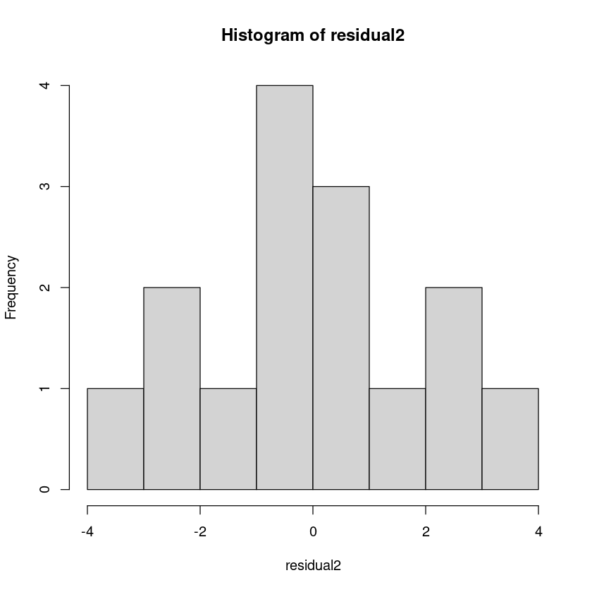
residual2 <- model2$residuals
head(residual2)
hist(residual2)

1: 0.345214860348173
2: 3.87452253360442
3: -2.64479086930799
4: -0.369359156300476
5: 1.07271444722616
6: 0.800293089055777

내적표준화된 잔차

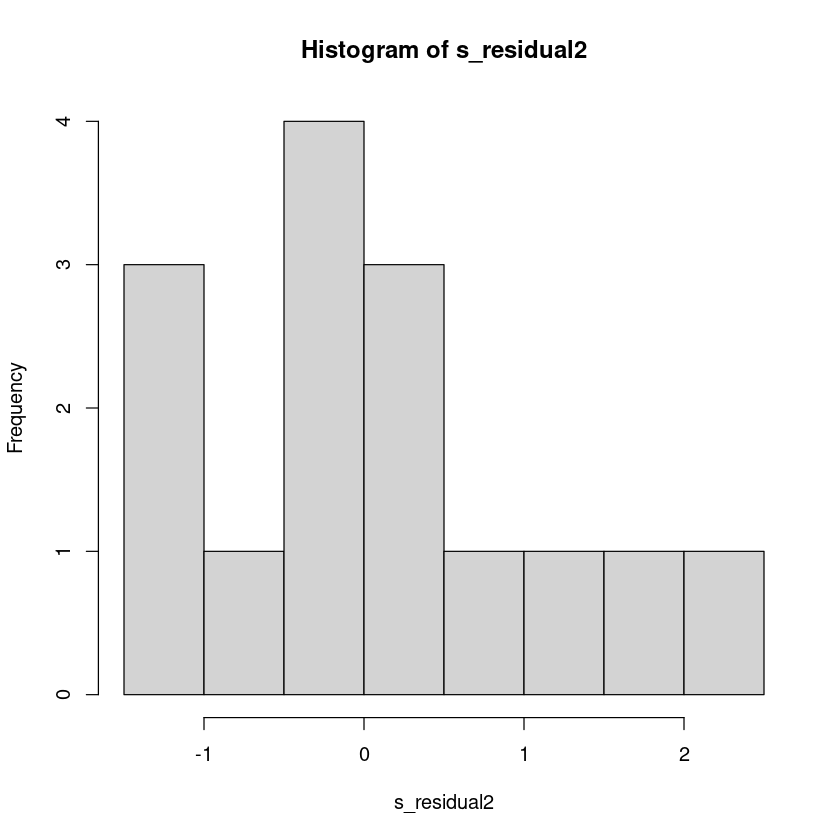
s_residual2 <- rstandard(model2)
head(s_residual2)
s_residual>2
hist(s_residual2)

1: 0.168693789872619
2: 2.04040961191812
3: -1.36846222178994
4: -0.192038604753614
5: 0.527462985239622
6: 0.470252444990339

1: FALSE
2: TRUE
3: FALSE
4: FALSE
5: FALSE
6: FALSE
7: FALSE
8: FALSE
9: FALSE
10: FALSE
11: FALSE
12: FALSE
13: FALSE
14: FALSE
15: FALSE

외적표준화된 잔차

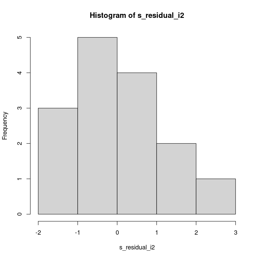
s_residual_i2 <- rstudent(model2)
head(s_residual_i2)
hist(s_residual_i2)

1: 0.161051677291382
2: 2.46770471155657
3: -1.43239034421095
4: -0.183409334396953
5: 0.509399466568036
6: 0.452944085994544

which.max(s_residual_i2)
s_residual_i[which.max(s_residual_i2)]

2: 2

2: 3.5482500706297

qt(0.975, 15-3-2)

2.22813885198627

$|r_i^*| \geq t_{\alpha/2}(10)$ 이므로 2번째 관측값은 유의수준 0.05에서 이상점이다.

영향점

influence(model2)

$hat

1: 0.229484482984878
2: 0.336559048244901
3: 0.312745387413974
4: 0.31935404183557
5: 0.238999578272863
6: 0.467111162145579
7: 0.176674868362933
8: 0.262199425033544
9: 0.414083032167575
10: 0.19055339953678
11: 0.0731668365931882
12: 0.174623444618773
13: 0.197413593761242
14: 0.241923572696132
15: 0.365108126332067

$coefficients

A matrix: 15 × 4 of type dbl
	(Intercept)	x1	x2	x3
1	0.95354693	0.0003764930	-5.561428e-03	-0.0014501180
2	-13.93952031	0.0672978312	8.377466e-02	-0.0248399264
3	4.69552573	-0.0704991936	-3.644734e-02	0.0705780525
4	0.50943934	0.0007684142	-5.873357e-03	0.0076533361
5	-2.27767961	0.0105499531	1.862708e-02	-0.0200833113
6	-4.18168476	-0.0332209276	3.130321e-02	0.0117532167
7	-2.20897093	0.0037053698	1.765648e-02	-0.0175478830
8	-0.01539851	0.0005690967	2.732094e-05	-0.0002319326
9	-0.51557236	-0.0263081084	9.369868e-03	-0.0028197702
10	0.12758711	0.0019405994	-7.974601e-04	-0.0013464759
11	-1.76717565	-0.0009954571	1.149237e-02	-0.0048224698
12	-0.86864768	-0.0001014964	7.037690e-03	-0.0060239702
13	2.27737859	-0.0219351895	-2.102859e-02	0.0439849174
14	3.66063758	0.0653541960	-2.631196e-02	-0.0454527846
15	13.67495355	-0.0124352729	-8.212831e-02	-0.0017947153

$sigma

1: 2.44193182869043
2: 1.92763082719566
3: 2.22726104086183
4: 2.44099449377856
5: 2.41397737377572
6: 2.42039452193581
7: 2.39715919509951
8: 2.44508463698753
9: 2.42314403118888
10: 2.44479643924596
11: 2.22712958167362
12: 2.43788055286261
13: 2.26047895469207
14: 2.20980300839363
15: 2.16577831202649

$wt.res

1: 0.345214860348173
2: 3.87452253360442
3: -2.64479086930799
4: -0.369359156300476
5: 1.07271444722616
6: 0.800293089055777
7: -1.38244275079492
8: -0.0208410556291935
9: -0.79131150566298
10: 0.109012275312978
11: -3.07226152705352
12: -0.539287518287805
13: 2.64051702167739
14: -2.88148775547281
15: 2.85950791128479

influence.measures(model2)

Influence measures of
     lm(formula = y ~ x1 + x2 + x3, data = dt) :

     dfb.1_    dfb.x1    dfb.x2   dfb.x3    dffit cov.r   cook.d    hat inf
1   0.06276  0.003172 -0.051979 -0.01524  0.08789 1.881 2.12e-03 0.2295    
2  -1.16230  0.718336  0.991882 -0.33074  1.75761 0.329 5.28e-01 0.3366   *
3   0.33885 -0.651274 -0.373479  0.81332 -0.96627 1.010 2.13e-01 0.3127    
4   0.03354  0.006477 -0.054915  0.08047 -0.12563 2.122 4.33e-03 0.3194   *
5  -0.15165  0.089922  0.176110 -0.21353  0.28547 1.737 2.18e-02 0.2390    
6  -0.27769 -0.282407  0.295171  0.12463  0.42407 2.533 4.85e-02 0.4671   *
7  -0.14811  0.031804  0.168104 -0.18788 -0.29442 1.518 2.29e-02 0.1767    
8  -0.00101  0.004789  0.000255 -0.00243 -0.00592 1.984 9.62e-06 0.2622    
9  -0.03420 -0.223389  0.088252 -0.02987 -0.35865 2.325 3.47e-02 0.4141   *
10  0.00839  0.016332 -0.007445 -0.01414  0.02405 1.807 1.59e-04 0.1906    
11 -0.12753 -0.009197  0.117770 -0.05558 -0.40259 0.748 3.70e-02 0.0732    
12 -0.05727 -0.000857  0.065885 -0.06342 -0.11200 1.732 3.43e-03 0.1746    
13  0.16193 -0.199660 -0.212315  0.49942  0.64667 0.973 9.83e-02 0.1974    
14  0.26625  0.608514 -0.271751 -0.52792 -0.84604 0.860 1.61e-01 0.2419    
15  1.01486 -0.118139 -0.865466 -0.02127  1.25657 0.874 3.41e-01 0.3651   *

DFFITS

dffits(model2)

1: 0.0878923790933185
2: 1.75761070078296
3: -0.966268917673672
4: -0.125631055448568
5: 0.285472714339999
6: 0.424068881254535
7: -0.294419313015607
8: -0.00591565303872599
9: -0.358654177245365
10: 0.0240465539273412
11: -0.402594900995498
12: -0.111997181258085
13: 0.646673748175155
14: -0.846036927571321
15: 1.25657461898781

which(abs(dffits(model2)) > 2*sqrt(2/(15-3-1)))

2: 2
3: 3
15: 15

Cook’s distance

cooks.distance(model2)

1: 0.00211889841023739
2: 0.527999760572049
3: 0.213048697653186
4: 0.00432581796350647
5: 0.0218442039453938
6: 0.0484602617041985
7: 0.0229122092214353
8: 9.62351672584315e-06
9: 0.0347416842517463
10: 0.000158976058928977
11: 0.0369801047117493
12: 0.00342909608500354
13: 0.0982906080447196
14: 0.160777911639787
15: 0.340678864434841

qf(0.5,3+1,15-3-1)

0.893156955577709

which(cooks.distance(model2) >qf(0.5,4,11))

없다

covratio

covratio(model2)

1: 1.88056935548212
2: 0.32929951279886
3: 1.0098427682077
4: 2.12234306958682
5: 1.73653332829024
6: 2.53311628226267
7: 1.51777046887204
8: 1.98433341199223
9: 2.32487827053021
10: 1.80699058897987
11: 0.748453434660152
12: 1.73240614043161
13: 0.973451691520289
14: 0.859642643137438
15: 0.873805339356644

which(abs(covratio(model2)-1) > 3*(3+1)/15)

1: 1
4: 4
6: 6
8: 8
9: 9
10: 10

정규성

shapiro.test(model2$residuals)


    Shapiro-Wilk normality test

data:  model2$residuals
W = 0.95818, p-value = 0.6608

회귀진단 그림

par(mfrow = c(2, 2))
plot(model2, pch=16)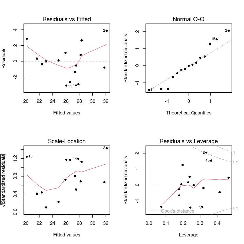

2번

어떤 화학공장에서 $NH_3$를 $HNO_3$로 산화시키는 공정을 가지고 있다. 이 산화공정에 미치는 중요한 요인으로 생각되어지는 변수는

$x_1$ = 작업속도

$x_2$ = 냉각수의 온도

$x_3$ = 흡수액 속의 $HNO_3$의 농도

이다. $y$는 $NH_3$를 $HNO_3$로 바꿀 때 손실되는 $NH_3$의 %로 잡아주었다. 21일간의 공정기간 중에 얻은 자료는 앞의 것과 같다.

실험번호	$x_1$	$x_2$	$x_3$	$y$
1	80	27	89	42
2	80	27	88	37
3	75	25	90	37
4	62	24	87	28
5	62	22	87	18
6	62	23	87	18
7	62	24	93	19
8	62	24	93	20
9	58	23	87	15
10	58	18	90	14
11	58	18	89	14
12	58	17	88	13
13	58	18	82	11
14	58	19	93	12
15	50	18	89	8
16	50	18	86	7
17	50	19	72	8
18	50	19	79	8
19	50	20	80	9
20	56	20	82	15
21	70	20	91	15

dt2 <- data.frame(x1 = c(80,80,75,62,62,62,62,62,58,58,58,58,58,58,50,50,50,50,50,56,70),
                 x2 = c(27,27,25,24,22,23,24,24,23,18,18,17,18,19,18,18,19,19,20,20,20),
                 x3 = c(89,88,90,87,87,87,93,93,87,90,89,88,82,93,89,86,72,79,80,82,91),
 y = c(42,37,37,28,18,18,19,20,15,14,14,13,11,12,8,7,8,8,9,15,15))

(1)

중회귀모형

$y_i = β_0 + β_1x_{i1} + β_2x_{i2} + β_3x_{i3} + ϵ_i$

$i = 1, 2, · · · , 21$

$ϵ_i $∼$N(0, σ^2_ϵ)$

이 데이터간의 관계를 설명하는 데 충분하다고 가정하고 다음의 물음에 답하시오. 유의수준 α = 0.05를 사용하여라.

pairs(dt2, pch=16)
cor(dt2)

A matrix: 4 × 4 of type dbl
	x1	x2	x3	y
x1	1.0000000	0.7818523	0.4885669	0.9196635
x2	0.7818523	1.0000000	0.3078454	0.8755044
x3	0.4885669	0.3078454	1.0000000	0.3776617
y	0.9196635	0.8755044	0.3776617	1.0000000

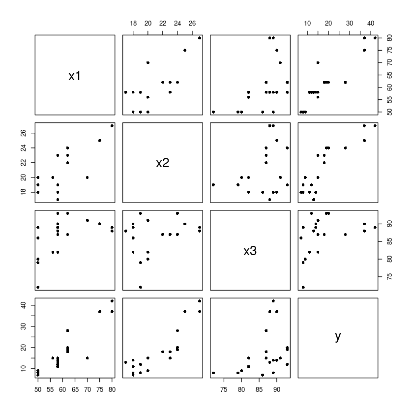
y와 x1의 상관관계가 높아보인다. y와 x2도 높아보이낟.
x1과 x2도 높다!!

m <- lm(y~., dt2) ##FM
summary(m)


Call:
lm(formula = y ~ ., data = dt2)

Residuals:
    Min      1Q  Median      3Q     Max 
-7.4829 -1.7449 -0.4688  2.3497  5.7224 

Coefficients:
            Estimate Std. Error t value Pr(>|t|)    
(Intercept) -42.5557    12.7798  -3.330 0.003965 ** 
x1            0.7107     0.1416   5.018 0.000106 ***
x2            1.2610     0.3768   3.347 0.003823 ** 
x3           -0.1092     0.1632  -0.669 0.512537    
---
Signif. codes:  0 ‘***’ 0.001 ‘**’ 0.01 ‘*’ 0.05 ‘.’ 0.1 ‘ ’ 1

Residual standard error: 3.289 on 17 degrees of freedom
Multiple R-squared:  0.9111,    Adjusted R-squared:  0.8954 
F-statistic: 58.08 on 3 and 17 DF,  p-value: 3.83e-09

(a)

add1/drop1 함수를 이용하여, 부분F검정통계량 값을 통한 후진제거법을 시행하여 가장 적절한 회귀모형을 구하여라.

drop1(m,test="F")

A anova: 4 × 6
	Df	Sum of Sq	RSS	AIC	F value	Pr(>F)
	<dbl>	<dbl>	<dbl>	<dbl>	<dbl>	<dbl>
<none>	NA	NA	183.9537	53.57340	NA	NA
x1	1	272.464536	456.4183	70.65663	25.1796878	0.0001055439
x2	1	121.206721	305.1604	62.20262	11.2012647	0.0038231136
x3	1	4.841619	188.7953	52.11896	0.4474361	0.5125370733

qf(0.95,1,21-3-1)

4.45132177246813

$F_L < F_{\alpha B}$ 이므로 설명변수 x3제거

m1 <- update(m, ~ . -x3)
summary(m1)


Call:
lm(formula = y ~ x1 + x2, data = dt2)

Residuals:
    Min      1Q  Median      3Q     Max 
-7.5290 -1.7505  0.1894  2.1156  5.6588 

Coefficients:
            Estimate Std. Error t value Pr(>|t|)    
(Intercept) -50.3588     5.1383  -9.801 1.22e-08 ***
x1            0.6712     0.1267   5.298 4.90e-05 ***
x2            1.2954     0.3675   3.525  0.00242 ** 
---
Signif. codes:  0 ‘***’ 0.001 ‘**’ 0.01 ‘*’ 0.05 ‘.’ 0.1 ‘ ’ 1

Residual standard error: 3.239 on 18 degrees of freedom
Multiple R-squared:  0.9088,    Adjusted R-squared:  0.8986 
F-statistic: 89.64 on 2 and 18 DF,  p-value: 4.382e-10

pvalue의 값도 유의하고 $R^2$도 약 90%의 설명력을 가진다. 각각의 회귀계수도 유의하다.
$y=-50.3588 + 0.6712 x_1 + 1.2954 x_2$

drop1(m1, test = "F")

A anova: 3 × 6
	Df	Sum of Sq	RSS	AIC	F value	Pr(>F)
	<dbl>	<dbl>	<dbl>	<dbl>	<dbl>	<dbl>
<none>	NA	NA	188.7953	52.11896	NA	NA
x1	1	294.3553	483.1506	69.85193	28.06423	0.0000489797
x2	1	130.3208	319.1161	61.14168	12.42496	0.0024191459

qf(0.95,1,21-2-1)

4.41387341917057

F-value값이 작은 x2를 제거하려고 봤더니 pr값이 0.002419로 유의하므로 제거하지 않는다.

(b)

add1/drop1 함수를 이용하여, 부분F검정통계량 값을 통한 전진선택법을 시행하여 가장 적절한 회귀모형을 구하여라.

m0 = lm(y ~ 1, data = dt2)
add1(m0, scope = y ~ x1 + x2 + x3, test = "F")

A anova: 4 × 6
	Df	Sum of Sq	RSS	AIC	F value	Pr(>F)
	<dbl>	<dbl>	<dbl>	<dbl>	<dbl>	<dbl>
<none>	NA	NA	2069.2381	98.39868	NA	NA
x1	1	1750.1220	319.1161	61.14168	104.201315	3.774296e-09
x2	1	1586.0875	483.1506	69.85193	62.373224	2.028017e-07
x3	1	295.1321	1774.1060	97.16712	3.160752	9.143800e-02

F값이 큰 x1을 추가하자. 심지어 유의하당

qf(0.95,1,21-1-1)

4.3807496923318

m1 <- update(m0, ~.+x1)
summary(m1)


Call:
lm(formula = y ~ x1, data = dt2)

Residuals:
     Min       1Q   Median       3Q      Max 
-12.2896  -1.1272  -0.0459   1.1166   8.8728 

Coefficients:
             Estimate Std. Error t value Pr(>|t|)    
(Intercept) -44.13202    6.10586  -7.228 7.31e-07 ***
x1            1.02031    0.09995  10.208 3.77e-09 ***
---
Signif. codes:  0 ‘***’ 0.001 ‘**’ 0.01 ‘*’ 0.05 ‘.’ 0.1 ‘ ’ 1

Residual standard error: 4.098 on 19 degrees of freedom
Multiple R-squared:  0.8458,    Adjusted R-squared:  0.8377 
F-statistic: 104.2 on 1 and 19 DF,  p-value: 3.774e-09

add1(m1,
 scope = y ~ x1 + x2 + x3,
 test = "F")

A anova: 3 × 6
	Df	Sum of Sq	RSS	AIC	F value	Pr(>F)
	<dbl>	<dbl>	<dbl>	<dbl>	<dbl>	<dbl>
<none>	NA	NA	319.1161	61.14168	NA	NA
x2	1	130.32077	188.7953	52.11896	12.4249569	0.002419146
x3	1	13.95567	305.1604	62.20262	0.8231803	0.376238733

x2의 Fvalue가 크고 유의하므로 추가하자.

m2 <- update(m1, ~ . +x2)
summary(m2)


Call:
lm(formula = y ~ x1 + x2, data = dt2)

Residuals:
    Min      1Q  Median      3Q     Max 
-7.5290 -1.7505  0.1894  2.1156  5.6588 

Coefficients:
            Estimate Std. Error t value Pr(>|t|)    
(Intercept) -50.3588     5.1383  -9.801 1.22e-08 ***
x1            0.6712     0.1267   5.298 4.90e-05 ***
x2            1.2954     0.3675   3.525  0.00242 ** 
---
Signif. codes:  0 ‘***’ 0.001 ‘**’ 0.01 ‘*’ 0.05 ‘.’ 0.1 ‘ ’ 1

Residual standard error: 3.239 on 18 degrees of freedom
Multiple R-squared:  0.9088,    Adjusted R-squared:  0.8986 
F-statistic: 89.64 on 2 and 18 DF,  p-value: 4.382e-10

add1(m2,
 scope = y ~ x1 + x2 + x3,
 test = "F")

A anova: 2 × 6
	Df	Sum of Sq	RSS	AIC	F value	Pr(>F)
	<dbl>	<dbl>	<dbl>	<dbl>	<dbl>	<dbl>
<none>	NA	NA	188.7953	52.11896	NA	NA
x3	1	4.841619	183.9537	53.57340	0.4474361	0.5125371

x3의 pr값도 유의수준 0.05에서 유의하지 않다. 모형에 포함될 수 없으므로 멈춘다. 최종모형은 x1과 x2를 포함한 모형이다.

(c)

add1/drop1 함수를 이용하여, 부분F검정통계량 값을 통한 단계적 전진선택법을 시행하여 가장 적절한 회귀모형을 구하여라.

m0 = lm(y ~ 1, data = dt2)

add1(m0,
 scope = y ~ x1 + x2 + x3,
 test = "F")

A anova: 4 × 6
	Df	Sum of Sq	RSS	AIC	F value	Pr(>F)
	<dbl>	<dbl>	<dbl>	<dbl>	<dbl>	<dbl>
<none>	NA	NA	2069.2381	98.39868	NA	NA
x1	1	1750.1220	319.1161	61.14168	104.201315	3.774296e-09
x2	1	1586.0875	483.1506	69.85193	62.373224	2.028017e-07
x3	1	295.1321	1774.1060	97.16712	3.160752	9.143800e-02

Fvalue가 크고 pr값이 유의하 x1을 추가하자.

m1 <- update(m0, ~ . +x1)
summary(m1)


Call:
lm(formula = y ~ x1, data = dt2)

Residuals:
     Min       1Q   Median       3Q      Max 
-12.2896  -1.1272  -0.0459   1.1166   8.8728 

Coefficients:
             Estimate Std. Error t value Pr(>|t|)    
(Intercept) -44.13202    6.10586  -7.228 7.31e-07 ***
x1            1.02031    0.09995  10.208 3.77e-09 ***
---
Signif. codes:  0 ‘***’ 0.001 ‘**’ 0.01 ‘*’ 0.05 ‘.’ 0.1 ‘ ’ 1

Residual standard error: 4.098 on 19 degrees of freedom
Multiple R-squared:  0.8458,    Adjusted R-squared:  0.8377 
F-statistic: 104.2 on 1 and 19 DF,  p-value: 3.774e-09

add1(m1,
 scope = y ~ x1 + x2 + x3,
 test = "F")

A anova: 3 × 6
	Df	Sum of Sq	RSS	AIC	F value	Pr(>F)
	<dbl>	<dbl>	<dbl>	<dbl>	<dbl>	<dbl>
<none>	NA	NA	319.1161	61.14168	NA	NA
x2	1	130.32077	188.7953	52.11896	12.4249569	0.002419146
x3	1	13.95567	305.1604	62.20262	0.8231803	0.376238733

x2의 Fvalue가 더 크고 pr값이 유의하므로 x2선택

m2 <- update(m1, ~ . +x2)

x1이 있는 모형에 x2를 추가함

drop1(m2, test = "F")

A anova: 3 × 6
	Df	Sum of Sq	RSS	AIC	F value	Pr(>F)
	<dbl>	<dbl>	<dbl>	<dbl>	<dbl>	<dbl>
<none>	NA	NA	188.7953	52.11896	NA	NA
x1	1	294.3553	483.1506	69.85193	28.06423	0.0000489797
x2	1	130.3208	319.1161	61.14168	12.42496	0.0024191459

x1을 보자. 제거할까? 유의하므로 제거하지 말자.

add1(m2,
 scope = y ~ x1 + x2 + x3,
 test = "F")

A anova: 2 × 6
	Df	Sum of Sq	RSS	AIC	F value	Pr(>F)
	<dbl>	<dbl>	<dbl>	<dbl>	<dbl>	<dbl>
<none>	NA	NA	188.7953	52.11896	NA	NA
x3	1	4.841619	183.9537	53.57340	0.4474361	0.5125371

유의수준 0.05에서는 유의하지 않으므로 x3를 추가하지 않는다.

summary(m2)


Call:
lm(formula = y ~ x1 + x2, data = dt2)

Residuals:
    Min      1Q  Median      3Q     Max 
-7.5290 -1.7505  0.1894  2.1156  5.6588 

Coefficients:
            Estimate Std. Error t value Pr(>|t|)    
(Intercept) -50.3588     5.1383  -9.801 1.22e-08 ***
x1            0.6712     0.1267   5.298 4.90e-05 ***
x2            1.2954     0.3675   3.525  0.00242 ** 
---
Signif. codes:  0 ‘***’ 0.001 ‘**’ 0.01 ‘*’ 0.05 ‘.’ 0.1 ‘ ’ 1

Residual standard error: 3.239 on 18 degrees of freedom
Multiple R-squared:  0.9088,    Adjusted R-squared:  0.8986 
F-statistic: 89.64 on 2 and 18 DF,  p-value: 4.382e-10

(2)

leaps 패키지의 regsubsets 함수를 이용하여, 다음의 물음에 답하여라.

library(leaps)

(a)

전역탐색법을 사용하여, 가능한 모든 회귀모형에 대하여 $MSE_p, R^2_p, R^2_{adj,p}, C_p$ 를 구하여라. (regsubsets 사용시, 옵션에서 nbest=1 대신에 적당한 숫자를 입력하면 모든 회귀모형에 대한 결과를 확인할 수 있다.)

fit<-regsubsets(y~., data=dt2, nbest=6,
method='exhaustive',
)
summary(fit)
with(summary(fit),
     round(cbind(which,rss,rsq,adjr2,cp,bic),3))

Subset selection object
Call: regsubsets.formula(y ~ ., data = dt2, nbest = 6, method = "exhaustive", 
    )
3 Variables  (and intercept)
   Forced in Forced out
x1     FALSE      FALSE
x2     FALSE      FALSE
x3     FALSE      FALSE
6 subsets of each size up to 3
Selection Algorithm: exhaustive
         x1  x2  x3 
1  ( 1 ) "*" " " " "
1  ( 2 ) " " "*" " "
1  ( 3 ) " " " " "*"
2  ( 1 ) "*" "*" " "
2  ( 2 ) "*" " " "*"
2  ( 3 ) " " "*" "*"
3  ( 1 ) "*" "*" "*"

A matrix: 7 × 9 of type dbl
	(Intercept)	x1	x2	x3	rss	rsq	adjr2	cp	bic
1	1	1	0	0	319.116	0.846	0.838	12.491	-33.168
1	1	0	1	0	483.151	0.767	0.754	27.650	-24.458
1	1	0	0	1	1774.106	0.143	0.098	146.953	2.857
2	1	1	1	0	188.795	0.909	0.899	2.447	-41.146
2	1	1	0	1	305.160	0.853	0.836	13.201	-31.062
2	1	0	1	1	456.418	0.779	0.755	27.180	-22.608
3	1	1	1	1	183.954	0.911	0.895	4.000	-38.647

(b)

$p = 1, p = 2, p = 3$에서 각각 가장 적절한 회귀모형을 구하여라. (기준 : $R^2_p$)

p=1인 경우에 $R_2$ 값이 가장 큰(0.846) 모형을 선택한다. 즉 $y=\beta_0+\beta_1x_1$

p=2인 경우에는 $y=\beta_0+\beta_1x_1+\beta_2x_2$

p=3인 경우에는 $y=\beta_0+\beta_1x_1+\beta_2x_2+\beta_3x_3$

fit<-regsubsets(y~., data=dt2, nbest=1,
method='exhaustive',
)
summary(fit)
with(summary(fit),
     round(cbind(which,rss,rsq,adjr2,cp,bic),3))

Subset selection object
Call: regsubsets.formula(y ~ ., data = dt2, nbest = 1, method = "exhaustive", 
    )
3 Variables  (and intercept)
   Forced in Forced out
x1     FALSE      FALSE
x2     FALSE      FALSE
x3     FALSE      FALSE
1 subsets of each size up to 3
Selection Algorithm: exhaustive
         x1  x2  x3 
1  ( 1 ) "*" " " " "
2  ( 1 ) "*" "*" " "
3  ( 1 ) "*" "*" "*"

A matrix: 3 × 9 of type dbl
	(Intercept)	x1	x2	x3	rss	rsq	adjr2	cp	bic
1	1	1	0	0	319.116	0.846	0.838	12.491	-33.168
2	1	1	1	0	188.795	0.909	0.899	2.447	-41.146
3	1	1	1	1	183.954	0.911	0.895	4.000	-38.647

(c)

위에서 구한 모형 중 가장 적절한 회귀모형을 선택하여라.

adjr이 제일 높은 모형-> y=x1+x2

rss는 작은것이 제일 좋은데 3개를 선택한 모형은 원래 제일 작음.. x1 1개만 선택한 모형의 rss는 319이고 x1과 x2를 선택한 모형의 rss는 188로 급격히 감소함. x3까ㅣ 추가한것은 183으로 별차이가 없으므로 x1+x2를 선택한 모형을 고르는 것이 좋아보인다. bic값도 제일 낮음

(d)

$C_p$의 경우 $C_p ≤ p + 1$ 이면 좋은 모형으로 판정하고, 이를 만족할 때 변수의 수가 가장 적은 모형을 선택하는 것이 좋다고 알려져 있다. $C_p$ 를 이용했을 때, $p = 1, p = 2, p = 3$에서 각각 가장 좋은 모형을 선택하여라.

p=1일때는 x1선택한 모형이 제일작지만, cp>2이므로 좋은 모형이 아니다.

p=2일때는 x1+x2

p=3일때는 x1+x2+x3

fit<-regsubsets(y~., data=dt2, nbest=6,
method='exhaustive',
)
summary(fit)
with(summary(fit),
     round(cbind(which,rss,rsq,adjr2,cp,bic),3))

Subset selection object
Call: regsubsets.formula(y ~ ., data = dt2, nbest = 6, method = "exhaustive", 
    )
3 Variables  (and intercept)
   Forced in Forced out
x1     FALSE      FALSE
x2     FALSE      FALSE
x3     FALSE      FALSE
6 subsets of each size up to 3
Selection Algorithm: exhaustive
         x1  x2  x3 
1  ( 1 ) "*" " " " "
1  ( 2 ) " " "*" " "
1  ( 3 ) " " " " "*"
2  ( 1 ) "*" "*" " "
2  ( 2 ) "*" " " "*"
2  ( 3 ) " " "*" "*"
3  ( 1 ) "*" "*" "*"

A matrix: 7 × 9 of type dbl
	(Intercept)	x1	x2	x3	rss	rsq	adjr2	cp	bic
1	1	1	0	0	319.116	0.846	0.838	12.491	-33.168
1	1	0	1	0	483.151	0.767	0.754	27.650	-24.458
1	1	0	0	1	1774.106	0.143	0.098	146.953	2.857
2	1	1	1	0	188.795	0.909	0.899	2.447	-41.146
2	1	1	0	1	305.160	0.853	0.836	13.201	-31.062
2	1	0	1	1	456.418	0.779	0.755	27.180	-22.608
3	1	1	1	1	183.954	0.911	0.895	4.000	-38.647

(e)

위에서 선택한 모형 중 $C_p$를 기준으로 가장 적절한 회귀모형을 선택하여라

p=2일때 x1+x2를 선택한 모형이 가장 적절하다. p=1인 경우에는 cp<p+1이므로 좋은 모형이라고 할 수 없다.

(3)

일차 선형항(lenear terms)만으로는 충분하지 않다고 생각하고 이차다항회귀모형

$y = β_0 + β_1x_1 + β_2x_2 + β_3x_3 + β_4x^2_1 + β_5x^2_2 + β_6x^2_3 + β_7x_1x_2 + β_8x_1x_3 + β_9x_2x_3 + ϵ$을 가정하였다. 다음 물음에 답하여라.

dt2$x_1 <- dt2$x1^2
dt2$x_2 <- dt2$x2^2
dt2$x_3 <- dt2$x3^2
dt2$x1x2 <- dt2$x1 * dt2$x2
dt2$x1x3 <- dt2$x1 * dt2$x1
dt2$x2x3 <- dt2$x2 * dt2$x3
head(dt2)

A data.frame: 6 × 10
	x1	x2	x3	y	x_1	x_2	x_3	x1x2	x1x3	x2x3
	<dbl>	<dbl>	<dbl>	<dbl>	<dbl>	<dbl>	<dbl>	<dbl>	<dbl>	<dbl>
1	80	27	89	42	6400	729	7921	2160	6400	2403
2	80	27	88	37	6400	729	7744	2160	6400	2376
3	75	25	90	37	5625	625	8100	1875	5625	2250
4	62	24	87	28	3844	576	7569	1488	3844	2088
5	62	22	87	18	3844	484	7569	1364	3844	1914
6	62	23	87	18	3844	529	7569	1426	3844	2001

(a)

변수간 상관계수를 구하여라.

cor(dt2)

A matrix: 10 × 10 of type dbl
	x1	x2	x3	y	x_1	x_2	x_3	x1x2	x1x3	x2x3
x1	1.0000000	0.7818523	0.4885669	0.9196635	0.9969709	0.8002266	0.4861833	0.9452829	0.9969709	0.8221139
x2	0.7818523	1.0000000	0.3078454	0.8755044	0.7846889	0.9982761	0.3079752	0.9377909	0.7846889	0.9542580
x3	0.4885669	0.3078454	1.0000000	0.3776617	0.4524089	0.3130881	0.9991718	0.4004805	0.4524089	0.5773637
y	0.9196635	0.8755044	0.3776617	1.0000000	0.9251379	0.8933751	0.3735385	0.9588371	0.9251379	0.8672805
x_1	0.9969709	0.7846889	0.4524089	0.9251379	1.0000000	0.8053207	0.4499860	0.9500453	1.0000000	0.8131868
x_2	0.8002266	0.9982761	0.3130881	0.8933751	0.8053207	1.0000000	0.3129003	0.9498899	0.8053207	0.9544366
x_3	0.4861833	0.3079752	0.9991718	0.3735385	0.4499860	0.3129003	1.0000000	0.3990206	0.4499860	0.5777549
x1x2	0.9452829	0.9377909	0.4004805	0.9588371	0.9500453	0.9498899	0.3990206	1.0000000	0.9500453	0.9290098
x1x3	0.9969709	0.7846889	0.4524089	0.9251379	1.0000000	0.8053207	0.4499860	0.9500453	1.0000000	0.8131868
x2x3	0.8221139	0.9542580	0.5773637	0.8672805	0.8131868	0.9544366	0.5777549	0.9290098	0.8131868	1.0000000

(b)

설명변수 9개를 모두 사용한 완전모형(full model)에 대한 분산분석표를 작성하고, α = 0.05에서 선형회귀모형의 유의성을 검정하시오.

model3 <- lm(y~.,data=dt2)
summary(model3)


Call:
lm(formula = y ~ ., data = dt2)

Residuals:
   Min     1Q Median     3Q    Max 
-4.265 -1.249  0.005  1.177  5.382 

Coefficients: (1 not defined because of singularities)
              Estimate Std. Error t value Pr(>|t|)
(Intercept) -95.454579 171.941017  -0.555    0.589
x1            1.918799   1.503723   1.276    0.226
x2           -4.101841  10.326442  -0.397    0.698
x3            1.727460   3.273516   0.528    0.607
x_1          -0.040497   0.026368  -1.536    0.151
x_2          -0.007079   0.265375  -0.027    0.979
x_3          -0.004630   0.023903  -0.194    0.850
x1x2          0.172153   0.128263   1.342    0.204
x1x3                NA         NA      NA       NA
x2x3         -0.054589   0.112622  -0.485    0.637

Residual standard error: 3.037 on 12 degrees of freedom
Multiple R-squared:  0.9465,    Adjusted R-squared:  0.9109 
F-statistic: 26.55 on 8 and 12 DF,  p-value: 1.706e-06

anova(model3)

A anova: 9 × 5
	Df	Sum Sq	Mean Sq	F value	Pr(>F)
	<int>	<dbl>	<dbl>	<dbl>	<dbl>
x1	1	1750.121989	1750.121989	189.7977744	1.023932e-08
x2	1	130.320772	130.320772	14.1330676	2.723908e-03
x3	1	4.841619	4.841619	0.5250654	4.825789e-01
x_1	1	8.498097	8.498097	0.9216043	3.559986e-01
x_2	1	39.533776	39.533776	4.2873712	6.062395e-02
x_3	1	5.206534	5.206534	0.5646399	4.668786e-01
x1x2	1	17.897053	17.897053	1.9409052	1.888401e-01
x2x3	1	2.166462	2.166462	0.2349492	6.366054e-01
Residuals	12	110.651792	9.220983	NA	NA

null_model <- lm(y~1, data=dt2)  #H0
model3<- lm(y~., data=dt2)  #H1

anova(null_model, model3)

A anova: 2 × 6
	Res.Df	RSS	Df	Sum of Sq	F	Pr(>F)
	<dbl>	<dbl>	<dbl>	<dbl>	<dbl>	<dbl>
1	20	2069.2381	NA	NA	NA	NA
2	12	110.6518	8	1958.586	26.55067	1.706475e-06

F=26.55067

(c)

상관계수들을 보고 변수를 하나만 선택할 때에는 어떤 변수가 선택될 것인지를 말하시오.

x1x3와 y의 상관계수가 0.9588371로 가장 높으므로 선택

(d)

상관계수들을 보고 변수를 하나만 제거시키려고 할 때, 어떤 변수가 제거될 것인가를 말할 수 있는가?

x3^2와 y의 상관계수가 0.3735385로 가장 작으므로 제거

(e)

add1/drop1 함수를 이용하여, $MSE_p$ 기준으로 단계적 전진선택법을 시행하여 가장 적절한 회귀모형을 구하여라.

model_step = step(
 m0,
 scope =y ~ x1 + x2 + x3+ I(x1^2)+I(x2^2)+I(x3^2)+I(x1*x2)+I(x1*x3)+I(x2*x3),
 direction = "both")
summary(model_step)

Start:  AIC=98.4
y ~ 1

             Df Sum of Sq     RSS    AIC
+ I(x1 * x2)  1   1902.39  166.85 47.523
+ I(x1^2)     1   1771.02  298.22 59.719
+ x1          1   1750.12  319.12 61.142
+ I(x2^2)     1   1651.50  417.74 66.797
+ x2          1   1586.09  483.15 69.852
+ I(x1 * x3)  1   1563.93  505.31 70.794
+ I(x2 * x3)  1   1556.43  512.81 71.103
+ x3          1    295.13 1774.11 97.167
+ I(x3^2)     1    288.72 1780.52 97.243
<none>                    2069.24 98.399

Step:  AIC=47.52
y ~ I(x1 * x2)

             Df Sum of Sq     RSS    AIC
<none>                     166.85 47.523
+ x2          1      9.63  157.22 48.275
+ I(x2 * x3)  1      8.34  158.51 48.447
+ I(x2^2)     1      6.42  160.42 48.699
+ I(x1^2)     1      4.28  162.56 48.977
+ x1          1      3.43  163.41 49.087
+ I(x1 * x3)  1      0.61  166.23 49.446
+ I(x3^2)     1      0.20  166.64 49.498
+ x3          1      0.10  166.75 49.511
- I(x1 * x2)  1   1902.39 2069.24 98.399


Call:
lm(formula = y ~ I(x1 * x2), data = dt2)

Residuals:
    Min      1Q  Median      3Q     Max 
-5.1481 -2.3759 -0.6042  2.6123  5.6241 

Coefficients:
             Estimate Std. Error t value Pr(>|t|)    
(Intercept) -15.29308    2.32149  -6.588 2.64e-06 ***
I(x1 * x2)    0.02532    0.00172  14.719 7.68e-12 ***
---
Signif. codes:  0 ‘***’ 0.001 ‘**’ 0.01 ‘*’ 0.05 ‘.’ 0.1 ‘ ’ 1

Residual standard error: 2.963 on 19 degrees of freedom
Multiple R-squared:  0.9194,    Adjusted R-squared:  0.9151 
F-statistic: 216.6 on 1 and 19 DF,  p-value: 7.675e-12

AIC로 확인해보니까 $y$~$I(x1*x2)$가 최종모형

m0 = lm(y ~ 1, data = dt2)
add1(m0,
 scope = y ~ x1 + x2 + x3+ I(x1^2)+I(x2^2)+I(x3^2)+I(x1*x2)+I(x1*x3)+I(x2*x3),
 test = "F")

A anova: 10 × 6
	Df	Sum of Sq	RSS	AIC	F value	Pr(>F)
	<dbl>	<dbl>	<dbl>	<dbl>	<dbl>	<dbl>
<none>	NA	NA	2069.2381	98.39868	NA	NA
x1	1	1750.1220	319.1161	61.14168	104.201315	3.774296e-09
x2	1	1586.0875	483.1506	69.85193	62.373224	2.028017e-07
x3	1	295.1321	1774.1060	97.16712	3.160752	9.143800e-02
I(x1^2)	1	1771.0198	298.2182	59.71937	112.834735	1.972872e-09
I(x2^2)	1	1651.4985	417.7396	66.79705	75.114902	5.001792e-08
I(x3^2)	1	288.7229	1780.5152	97.24285	3.080982	9.532366e-02
I(x1 * x2)	1	1902.3924	166.8457	47.52349	216.639964	7.675449e-12
I(x1 * x3)	1	1563.9280	505.3101	70.79365	58.804744	3.124530e-07
I(x2 * x3)	1	1556.4302	512.8079	71.10295	57.667163	3.601417e-07

qf(0.95,1,21-9-1)

4.84433567494361

RSS의 값이 가장 작은 x1*x2 변수를 선택

m1 <- update(m0, ~ . +I(x1*x2))
summary(m1)


Call:
lm(formula = y ~ I(x1 * x2), data = dt2)

Residuals:
    Min      1Q  Median      3Q     Max 
-5.1481 -2.3759 -0.6042  2.6123  5.6241 

Coefficients:
             Estimate Std. Error t value Pr(>|t|)    
(Intercept) -15.29308    2.32149  -6.588 2.64e-06 ***
I(x1 * x2)    0.02532    0.00172  14.719 7.68e-12 ***
---
Signif. codes:  0 ‘***’ 0.001 ‘**’ 0.01 ‘*’ 0.05 ‘.’ 0.1 ‘ ’ 1

Residual standard error: 2.963 on 19 degrees of freedom
Multiple R-squared:  0.9194,    Adjusted R-squared:  0.9151 
F-statistic: 216.6 on 1 and 19 DF,  p-value: 7.675e-12

add1(m1, 
     scope = y ~ x1 + x2 + x3+ I(x1^2)+I(x2^2)+I(x3^2)+I(x1*x2)+I(x1*x3)+I(x2*x3),
 test = "F")

A anova: 9 × 6
	Df	Sum of Sq	RSS	AIC	F value	Pr(>F)
	<dbl>	<dbl>	<dbl>	<dbl>	<dbl>	<dbl>
<none>	NA	NA	166.8457	47.52349	NA	NA
x1	1	3.43425436	163.4115	49.08673	0.37828785	0.5462188
x2	1	9.62876230	157.2170	48.27519	1.10241098	0.3076309
x3	1	0.09886847	166.7469	49.51104	0.01067266	0.9188604
I(x1^2)	1	4.28275838	162.5630	48.97740	0.47421406	0.4998351
I(x2^2)	1	6.42241880	160.4233	48.69917	0.72061555	0.4070905
I(x3^2)	1	0.20188867	166.6438	49.49807	0.02180696	0.8842434
I(x1 * x3)	1	0.61479960	166.2309	49.44597	0.06657240	0.7993213
I(x2 * x3)	1	8.33654778	158.5092	48.44709	0.94668239	0.3434600

qf(0.95,1,21-8-1)

4.74722534672251

X2의 RSS값이 157.2170으로 가장 낮지만 pr값이 유의하지 않으므로 선택하지 않는다.

(f)

regsubsets 함수를 이용하여 전역탐색법을 시행하여라. $C_p, MSE_p, R^2_{adj,p}$ 기준으로 가장 적절한 모형을 선택한 후 위의 결과와 비교하시오

fit2 <- regsubsets(y~., data=dt2, nbest=20, method='exhaustive',)
summary(fit2)

Warning message in leaps.setup(x, y, wt = wt, nbest = nbest, nvmax = nvmax, force.in = force.in, :
“1  linear dependencies found”

Reordering variables and trying again:

Subset selection object
Call: regsubsets.formula(y ~ ., data = dt2, nbest = 20, method = "exhaustive", 
    )
9 Variables  (and intercept)
     Forced in Forced out
x1       FALSE      FALSE
x2       FALSE      FALSE
x3       FALSE      FALSE
x_1      FALSE      FALSE
x_2      FALSE      FALSE
x_3      FALSE      FALSE
x1x2     FALSE      FALSE
x2x3     FALSE      FALSE
x1x3     FALSE      FALSE
20 subsets of each size up to 8
Selection Algorithm: exhaustive
          x1  x2  x3  x_1 x_2 x_3 x1x2 x1x3 x2x3
1  ( 1 )  " " " " " " " " " " " " "*"  " "  " " 
1  ( 2 )  " " " " " " " " " " " " " "  "*"  " " 
1  ( 3 )  " " " " " " "*" " " " " " "  " "  " " 
1  ( 4 )  "*" " " " " " " " " " " " "  " "  " " 
1  ( 5 )  " " " " " " " " "*" " " " "  " "  " " 
1  ( 6 )  " " "*" " " " " " " " " " "  " "  " " 
1  ( 7 )  " " " " " " " " " " " " " "  " "  "*" 
1  ( 8 )  " " " " "*" " " " " " " " "  " "  " " 
1  ( 9 )  " " " " " " " " " " "*" " "  " "  " " 
2  ( 1 )  " " "*" " " " " " " " " "*"  " "  " " 
2  ( 2 )  " " " " " " " " " " " " "*"  " "  "*" 
2  ( 3 )  " " " " " " " " "*" " " "*"  " "  " " 
2  ( 4 )  " " " " " " " " " " " " "*"  "*"  " " 
2  ( 5 )  " " " " " " "*" " " " " "*"  " "  " " 
2  ( 6 )  "*" " " " " " " " " " " "*"  " "  " " 
2  ( 7 )  " " " " " " " " " " "*" "*"  " "  " " 
2  ( 8 )  " " " " "*" " " " " " " "*"  " "  " " 
2  ( 9 )  " " " " " " " " "*" " " " "  "*"  " " 
2  ( 10 ) " " " " " " "*" "*" " " " "  " "  " " 
2  ( 11 ) "*" " " " " " " "*" " " " "  " "  " " 
2  ( 12 ) " " "*" " " " " " " " " " "  "*"  " " 
2  ( 13 ) " " "*" " " "*" " " " " " "  " "  " " 
2  ( 14 ) "*" "*" " " " " " " " " " "  " "  " " 
2  ( 15 ) " " " " " " " " " " " " " "  "*"  "*" 
2  ( 16 ) " " " " " " "*" " " " " " "  " "  "*" 
2  ( 17 ) "*" " " " " " " " " " " " "  " "  "*" 
2  ( 18 ) " " "*" " " " " "*" " " " "  " "  " " 
2  ( 19 ) " " " " " " " " " " "*" " "  "*"  " " 
2  ( 20 ) " " " " " " "*" " " "*" " "  " "  " " 
3  ( 1 )  " " "*" " " "*" " " " " "*"  " "  " " 
3  ( 2 )  " " "*" " " " " " " " " "*"  "*"  " " 
3  ( 3 )  " " " " " " "*" "*" " " "*"  " "  " " 
3  ( 4 )  " " " " " " " " "*" " " "*"  "*"  " " 
3  ( 5 )  "*" "*" " " " " "*" " " " "  " "  " " 
3  ( 6 )  " " "*" " " " " "*" " " "*"  " "  " " 
3  ( 7 )  " " "*" " " "*" "*" " " " "  " "  " " 
3  ( 8 )  " " "*" " " " " "*" " " " "  "*"  " " 
3  ( 9 )  "*" "*" " " " " " " " " "*"  " "  " " 
3  ( 10 ) " " " " "*" " " " " " " "*"  " "  "*" 
3  ( 11 ) " " " " " " " " " " "*" "*"  " "  "*" 
3  ( 12 ) " " "*" " " " " " " " " "*"  " "  "*" 
3  ( 13 ) " " "*" " " " " " " "*" "*"  " "  " " 
3  ( 14 ) " " "*" "*" " " " " " " "*"  " "  " " 
3  ( 15 ) "*" " " " " " " "*" " " "*"  " "  " " 
3  ( 16 ) " " " " "*" " " " " "*" "*"  " "  " " 
3  ( 17 ) " " " " " " " " "*" " " "*"  " "  "*" 
3  ( 18 ) "*" " " " " " " " " " " "*"  " "  "*" 
3  ( 19 ) " " " " " " " " " " " " "*"  "*"  "*" 
3  ( 20 ) " " " " " " "*" " " " " "*"  " "  "*" 
4  ( 1 )  "*" "*" " " " " " " " " "*"  "*"  " " 
4  ( 2 )  "*" "*" " " "*" " " " " "*"  " "  " " 
4  ( 3 )  " " " " "*" "*" " " " " "*"  " "  "*" 
4  ( 4 )  " " " " "*" " " " " " " "*"  "*"  "*" 
4  ( 5 )  " " "*" " " "*" "*" " " "*"  " "  " " 
4  ( 6 )  " " "*" " " " " "*" " " "*"  "*"  " " 
4  ( 7 )  " " " " " " "*" " " "*" "*"  " "  "*" 
4  ( 8 )  " " " " " " " " " " "*" "*"  "*"  "*" 
4  ( 9 )  " " "*" "*" "*" " " " " "*"  " "  " " 
4  ( 10 ) " " "*" "*" " " " " " " "*"  "*"  " " 
4  ( 11 ) " " "*" " " "*" " " " " "*"  " "  "*" 
4  ( 12 ) " " "*" " " " " " " " " "*"  "*"  "*" 
4  ( 13 ) " " "*" " " " " " " "*" "*"  "*"  " " 
4  ( 14 ) " " "*" " " "*" " " "*" "*"  " "  " " 
4  ( 15 ) " " "*" " " "*" " " " " "*"  "*"  " " 
4  ( 16 ) "*" " " "*" " " "*" " " " "  " "  "*" 
4  ( 17 ) "*" " " " " " " "*" " " "*"  "*"  " " 
4  ( 18 ) "*" " " " " "*" "*" " " "*"  " "  " " 
4  ( 19 ) " " " " "*" " " "*" " " "*"  " "  "*" 
4  ( 20 ) " " " " " " "*" "*" " " "*"  " "  "*" 
5  ( 1 )  "*" " " "*" "*" " " " " "*"  " "  "*" 
5  ( 2 )  "*" " " "*" " " " " " " "*"  "*"  "*" 
5  ( 3 )  "*" " " " " " " " " "*" "*"  "*"  "*" 
5  ( 4 )  "*" " " " " "*" " " "*" "*"  " "  "*" 
5  ( 5 )  "*" "*" " " "*" " " " " "*"  " "  "*" 
5  ( 6 )  "*" "*" " " " " " " " " "*"  "*"  "*" 
5  ( 7 )  "*" "*" " " "*" " " "*" "*"  " "  " " 
5  ( 8 )  "*" "*" " " " " " " "*" "*"  "*"  " " 
5  ( 9 )  "*" "*" "*" " " " " " " "*"  "*"  " " 
5  ( 10 ) "*" "*" "*" "*" " " " " "*"  " "  " " 
5  ( 11 ) "*" "*" " " "*" "*" " " "*"  " "  " " 
5  ( 12 ) "*" "*" " " " " "*" " " "*"  "*"  " " 
5  ( 13 ) "*" "*" " " "*" " " " " "*"  "*"  " " 
5  ( 14 ) " " " " "*" " " " " "*" "*"  "*"  "*" 
5  ( 15 ) " " " " "*" "*" " " "*" "*"  " "  "*" 
5  ( 16 ) " " " " "*" " " "*" " " "*"  "*"  "*" 
5  ( 17 ) " " " " "*" "*" "*" " " "*"  " "  "*" 
5  ( 18 ) " " "*" "*" "*" " " " " "*"  " "  "*" 
5  ( 19 ) " " "*" "*" " " " " " " "*"  "*"  "*" 
5  ( 20 ) " " " " "*" "*" " " " " "*"  "*"  "*" 
6  ( 1 )  "*" "*" "*" " " " " " " "*"  "*"  "*" 
6  ( 2 )  "*" "*" "*" "*" " " " " "*"  " "  "*" 
6  ( 3 )  "*" " " "*" " " "*" " " "*"  "*"  "*" 
6  ( 4 )  "*" " " "*" "*" "*" " " "*"  " "  "*" 
6  ( 5 )  "*" " " "*" "*" " " "*" "*"  " "  "*" 
6  ( 6 )  "*" " " "*" " " " " "*" "*"  "*"  "*" 
6  ( 7 )  "*" " " "*" "*" " " " " "*"  "*"  "*" 
6  ( 8 )  "*" "*" "*" " " " " "*" "*"  "*"  " " 
6  ( 9 )  "*" "*" "*" "*" " " "*" "*"  " "  " " 
6  ( 10 ) "*" "*" " " "*" " " "*" "*"  " "  "*" 
6  ( 11 ) "*" "*" " " " " " " "*" "*"  "*"  "*" 
6  ( 12 ) "*" " " " " " " "*" "*" "*"  "*"  "*" 
6  ( 13 ) "*" " " " " "*" "*" "*" "*"  " "  "*" 
6  ( 14 ) "*" " " " " "*" " " "*" "*"  "*"  "*" 
6  ( 15 ) "*" "*" " " "*" "*" " " "*"  " "  "*" 
6  ( 16 ) "*" "*" " " " " "*" " " "*"  "*"  "*" 
6  ( 17 ) "*" "*" " " "*" " " " " "*"  "*"  "*" 
6  ( 18 ) "*" "*" " " "*" "*" "*" "*"  " "  " " 
6  ( 19 ) "*" "*" " " " " "*" "*" "*"  "*"  " " 
6  ( 20 ) "*" "*" " " "*" " " "*" "*"  "*"  " " 
7  ( 1 )  "*" "*" "*" " " " " "*" "*"  "*"  "*" 
7  ( 2 )  "*" "*" "*" "*" " " "*" "*"  " "  "*" 
7  ( 3 )  "*" "*" "*" " " "*" " " "*"  "*"  "*" 
7  ( 4 )  "*" "*" "*" "*" "*" " " "*"  " "  "*" 
7  ( 5 )  "*" "*" "*" "*" " " " " "*"  "*"  "*" 
7  ( 6 )  "*" " " "*" " " "*" "*" "*"  "*"  "*" 
7  ( 7 )  "*" " " "*" "*" "*" "*" "*"  " "  "*" 
7  ( 8 )  "*" " " "*" "*" "*" " " "*"  "*"  "*" 
7  ( 9 )  "*" " " "*" "*" " " "*" "*"  "*"  "*" 
7  ( 10 ) "*" "*" "*" " " "*" "*" "*"  "*"  " " 
7  ( 11 ) "*" "*" "*" "*" "*" "*" "*"  " "  " " 
7  ( 12 ) "*" "*" "*" "*" " " "*" "*"  "*"  " " 
7  ( 13 ) "*" "*" " " "*" "*" "*" "*"  " "  "*" 
7  ( 14 ) "*" "*" " " " " "*" "*" "*"  "*"  "*" 
7  ( 15 ) "*" "*" " " "*" " " "*" "*"  "*"  "*" 
7  ( 16 ) "*" " " " " "*" "*" "*" "*"  "*"  "*" 
7  ( 17 ) "*" "*" " " "*" "*" " " "*"  "*"  "*" 
7  ( 18 ) "*" "*" " " "*" "*" "*" "*"  "*"  " " 
7  ( 19 ) "*" "*" "*" "*" "*" " " "*"  "*"  " " 
7  ( 20 ) " " "*" "*" " " "*" "*" "*"  "*"  "*" 
8  ( 1 )  "*" "*" "*" " " "*" "*" "*"  "*"  "*" 
8  ( 2 )  "*" "*" "*" "*" "*" "*" "*"  " "  "*" 
8  ( 3 )  "*" "*" "*" "*" " " "*" "*"  "*"  "*" 
8  ( 4 )  "*" "*" "*" "*" "*" " " "*"  "*"  "*" 
8  ( 5 )  "*" " " "*" "*" "*" "*" "*"  "*"  "*" 
8  ( 6 )  "*" "*" " " "*" "*" "*" "*"  "*"  "*" 
8  ( 7 )  " " "*" "*" "*" "*" "*" "*"  "*"  "*" 
8  ( 8 )  "*" "*" "*" "*" "*" "*" " "  "*"  "*"

with(summary(fit2),
     round(cbind(which,rss,rsq,adjr2,cp,bic),3))

A matrix: 137 × 15 of type dbl
	(Intercept)	x1	x2	x3	x_1	x_2	x_3	x1x2	x1x3	x2x3	rss	rsq	adjr2	cp	bic
1	1	0	0	0	0	0	0	1	0	0	166.846	0.919	0.915	-0.414	-46.786
1	1	0	0	0	0	0	0	0	1	0	298.218	0.856	0.848	12.646	-34.590
1	1	0	0	0	1	0	0	0	0	0	298.218	0.856	0.848	12.646	-34.590
1	1	1	0	0	0	0	0	0	0	0	319.116	0.846	0.838	14.724	-33.168
1	1	0	0	0	0	1	0	0	0	0	417.740	0.798	0.787	24.528	-27.513
1	1	0	1	0	0	0	0	0	0	0	483.151	0.767	0.754	31.030	-24.458
1	1	0	0	0	0	0	0	0	0	1	512.808	0.752	0.739	33.979	-23.207
1	1	0	0	1	0	0	0	0	0	0	1774.106	0.143	0.098	159.366	2.857
1	1	0	0	0	0	0	1	0	0	0	1780.515	0.140	0.094	160.003	2.933
2	1	0	1	0	0	0	0	1	0	0	157.217	0.924	0.916	0.629	-44.990
2	1	0	0	0	0	0	0	1	0	1	158.509	0.923	0.915	0.758	-44.818
2	1	0	0	0	0	1	0	1	0	0	160.423	0.922	0.914	0.948	-44.566
2	1	0	0	0	0	0	0	1	1	0	162.563	0.921	0.913	1.161	-44.288
2	1	0	0	0	1	0	0	1	0	0	162.563	0.921	0.913	1.161	-44.288
2	1	1	0	0	0	0	0	1	0	0	163.411	0.921	0.912	1.245	-44.178
2	1	0	0	0	0	0	1	1	0	0	166.644	0.919	0.911	1.566	-43.767
2	1	0	0	1	0	0	0	1	0	0	166.747	0.919	0.910	1.576	-43.754
2	1	0	0	0	0	1	0	0	1	0	168.659	0.918	0.909	1.767	-43.515
2	1	0	0	0	1	1	0	0	0	0	168.659	0.918	0.909	1.767	-43.515
2	1	1	0	0	0	1	0	0	0	0	176.505	0.915	0.905	2.547	-42.560
2	1	0	1	0	0	0	0	0	1	0	177.768	0.914	0.905	2.672	-42.410
2	1	0	1	0	1	0	0	0	0	0	177.768	0.914	0.905	2.672	-42.410
2	1	1	1	0	0	0	0	0	0	0	188.795	0.909	0.899	3.768	-41.146
2	1	0	0	0	0	0	0	0	1	1	217.470	0.895	0.883	6.619	-38.177
2	1	0	0	0	1	0	0	0	0	1	217.470	0.895	0.883	6.619	-38.177
2	1	1	0	0	0	0	0	0	0	1	240.158	0.884	0.871	8.874	-36.093
2	1	0	1	0	0	1	0	0	0	0	257.547	0.876	0.862	10.603	-34.625
2	1	0	0	0	0	0	1	0	1	0	293.474	0.858	0.842	14.175	-31.883
2	1	0	0	0	1	0	1	0	0	0	293.474	0.858	0.842	14.175	-31.883
3	1	0	1	0	1	0	0	1	0	0	132.668	0.936	0.925	0.189	-45.511
⋮	⋮	⋮	⋮	⋮	⋮	⋮	⋮	⋮	⋮	⋮	⋮	⋮	⋮	⋮	⋮
6	1	1	1	0	0	1	1	1	1	0	115.569	0.944	0.920	4.489	-39.275
6	1	1	1	0	1	0	1	1	1	0	115.767	0.944	0.920	4.508	-39.239
7	1	1	1	1	0	0	1	1	1	1	110.658	0.947	0.918	6.001	-37.142
7	1	1	1	1	1	0	1	1	0	1	110.658	0.947	0.918	6.001	-37.142
7	1	1	1	1	0	1	0	1	1	1	110.998	0.946	0.917	6.034	-37.078
7	1	1	1	1	1	1	0	1	0	1	110.998	0.946	0.917	6.034	-37.078
7	1	1	1	1	1	0	0	1	1	1	110.998	0.946	0.917	6.034	-37.078
7	1	1	0	1	0	1	1	1	1	1	112.107	0.946	0.917	6.145	-36.869
7	1	1	0	1	1	1	1	1	0	1	112.107	0.946	0.917	6.145	-36.869
7	1	1	0	1	1	1	0	1	1	1	112.112	0.946	0.917	6.145	-36.868
7	1	1	0	1	1	0	1	1	1	1	112.246	0.946	0.917	6.158	-36.843
7	1	1	1	1	0	1	1	1	1	0	112.818	0.945	0.916	6.215	-36.736
7	1	1	1	1	1	1	1	1	0	0	112.818	0.945	0.916	6.215	-36.736
7	1	1	1	1	1	0	1	1	1	0	112.974	0.945	0.916	6.231	-36.707
7	1	1	1	0	1	1	1	1	0	1	113.220	0.945	0.916	6.255	-36.662
7	1	1	1	0	0	1	1	1	1	1	113.220	0.945	0.916	6.255	-36.662
7	1	1	1	0	1	0	1	1	1	1	113.233	0.945	0.916	6.257	-36.659
7	1	1	0	0	1	1	1	1	1	1	114.787	0.945	0.915	6.411	-36.373
7	1	1	1	0	1	1	0	1	1	1	115.049	0.944	0.914	6.437	-36.325
7	1	1	1	0	1	1	1	1	1	0	115.569	0.944	0.914	6.489	-36.230
7	1	1	1	1	1	1	0	1	1	0	115.969	0.944	0.914	6.529	-36.158
7	1	0	1	1	0	1	1	1	1	1	125.666	0.939	0.907	7.493	-34.471
8	1	1	1	1	0	1	1	1	1	1	110.652	0.947	0.911	8.000	-34.099
8	1	1	1	1	1	1	1	1	0	1	110.652	0.947	0.911	8.000	-34.099
8	1	1	1	1	1	0	1	1	1	1	110.658	0.947	0.911	8.001	-34.098
8	1	1	1	1	1	1	0	1	1	1	110.998	0.946	0.911	8.034	-34.033
8	1	1	0	1	1	1	1	1	1	1	112.107	0.946	0.910	8.145	-33.824
8	1	1	1	0	1	1	1	1	1	1	113.220	0.945	0.909	8.255	-33.617
8	1	0	1	1	1	1	1	1	1	1	125.666	0.939	0.899	9.493	-31.427
8	1	1	1	1	1	1	1	0	1	1	127.263	0.938	0.897	9.651	-31.162

cp기준으로는 x1x2를 선택한 변수 1개가 가장 적절하다.

fit3 <- regsubsets(y~., data=dt2, nbest=1, method='exhaustive',)
summary(fit3)
with(summary(fit3),
     round(cbind(which,rss,rsq,adjr2,cp,bic),3))

Warning message in leaps.setup(x, y, wt = wt, nbest = nbest, nvmax = nvmax, force.in = force.in, :
“1  linear dependencies found”

Reordering variables and trying again:

Subset selection object
Call: regsubsets.formula(y ~ ., data = dt2, nbest = 1, method = "exhaustive", 
    )
9 Variables  (and intercept)
     Forced in Forced out
x1       FALSE      FALSE
x2       FALSE      FALSE
x3       FALSE      FALSE
x_1      FALSE      FALSE
x_2      FALSE      FALSE
x_3      FALSE      FALSE
x1x2     FALSE      FALSE
x2x3     FALSE      FALSE
x1x3     FALSE      FALSE
1 subsets of each size up to 8
Selection Algorithm: exhaustive
         x1  x2  x3  x_1 x_2 x_3 x1x2 x1x3 x2x3
1  ( 1 ) " " " " " " " " " " " " "*"  " "  " " 
2  ( 1 ) " " "*" " " " " " " " " "*"  " "  " " 
3  ( 1 ) " " "*" " " " " " " " " "*"  "*"  " " 
4  ( 1 ) "*" "*" " " " " " " " " "*"  "*"  " " 
5  ( 1 ) "*" " " "*" "*" " " " " "*"  " "  "*" 
6  ( 1 ) "*" "*" "*" "*" " " " " "*"  " "  "*" 
7  ( 1 ) "*" "*" "*" "*" " " "*" "*"  " "  "*" 
8  ( 1 ) "*" "*" "*" "*" "*" "*" "*"  " "  "*"

A matrix: 8 × 15 of type dbl
	(Intercept)	x1	x2	x3	x_1	x_2	x_3	x1x2	x1x3	x2x3	rss	rsq	adjr2	cp	bic
1	1	0	0	0	0	0	0	1	0	0	166.846	0.919	0.915	-0.414	-46.786
2	1	0	1	0	0	0	0	1	0	0	157.217	0.924	0.916	0.629	-44.990
3	1	0	1	0	0	0	0	1	1	0	132.668	0.936	0.925	0.189	-45.511
4	1	1	1	0	0	0	0	1	1	0	120.807	0.942	0.927	1.009	-44.433
5	1	1	0	1	1	0	0	1	0	1	112.246	0.946	0.928	2.158	-42.932
6	1	1	1	1	1	0	0	1	0	1	110.998	0.946	0.923	4.034	-40.122
7	1	1	1	1	1	0	1	1	0	1	110.658	0.947	0.918	6.001	-37.142
8	1	1	1	1	1	1	1	1	0	1	110.652	0.947	0.911	8.000	-34.099

실험번호	\(x_1\)	\(x_2\)	\(x_3\)	\(y\)
1	80	27	89	42
2	80	27	88	37
3	75	25	90	37
4	62	24	87	28
5	62	22	87	18
6	62	23	87	18
7	62	24	93	19
8	62	24	93	20
9	58	23	87	15
10	58	18	90	14
11	58	18	89	14
12	58	17	88	13
13	58	18	82	11
14	58	19	93	12
15	50	18	89	8
16	50	18	86	7
17	50	19	72	8
18	50	19	79	8
19	50	20	80	9
20	56	20	82	15
21	70	20	91	15