10wk-038: 아이스크림 – 의사결정나무 원리

최규빈
2023-11-10

1. 강의영상

https://youtu.be/playlist?list=PLQqh36zP38-ypGHw375XVlBInqUzsxdd8&si=BWDa9FfxtVfYd6dj

2. Imports

import numpy as np
import pandas as pd
import matplotlib.pyplot as plt
import matplotlib.animation
import IPython
import sklearn.tree
#---#
import warnings
warnings.filterwarnings('ignore')

3. Data

np.random.seed(43052)
temp = pd.read_csv('https://raw.githubusercontent.com/guebin/DV2022/master/posts/temp.csv').iloc[:,3].to_numpy()[:100]
temp.sort()
eps = np.random.randn(100)*3 # 오차
icecream_sales = 20 + temp * 2.5 + eps 
df_train = pd.DataFrame({'temp':temp,'sales':icecream_sales})
df_train

	temp	sales
0	-4.1	10.900261
1	-3.7	14.002524
2	-3.0	15.928335
3	-1.3	17.673681
4	-0.5	19.463362
...	...	...
95	12.4	54.926065
96	13.4	54.716129
97	14.7	56.194791
98	15.0	60.666163
99	15.2	61.561043

100 rows × 2 columns

4. 의사결정나무 원리

A. 분할이 정해졌을때 \(\hat{y}\)을 결정하는 방법?

- step1~4

## step1
X = df_train[['temp']]
y = df_train['sales']
## step2
predictr = sklearn.tree.DecisionTreeRegressor(max_depth=1) 
## step3 
predictr.fit(X,y) 
## step4 -- pass 
# predictr.predict(X)

DecisionTreeRegressor(max_depth=1)

In a Jupyter environment, please rerun this cell to show the HTML representation or trust the notebook.
On GitHub, the HTML representation is unable to render, please try loading this page with nbviewer.org.

- tree 시각화 \(\to\) 분할파악

sklearn.tree.plot_tree(predictr)

[Text(0.5, 0.75, 'x[0] <= 5.05\nsquared_error = 111.946\nsamples = 100\nvalue = 33.973'),
 Text(0.25, 0.25, 'squared_error = 34.94\nsamples = 45\nvalue = 24.788'),
 Text(0.75, 0.25, 'squared_error = 49.428\nsamples = 55\nvalue = 41.489')]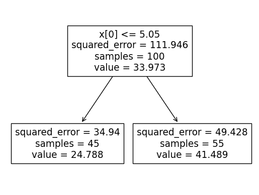

- 분할에 따른 \(\hat{y}\) 계산

df_train[df_train.temp<= 5.05].sales.mean(),df_train[df_train.temp> 5.05].sales.mean()

(24.787609205775055, 41.489079055828356)

B. 분할을 결정하는 방법?

- 예비학습

predictr.score(X,y)

0.6167038863844929

이 값이 내부적으로 어떻게 계산된거지?

predictr.score??

Signature: predictr.score(X, y, sample_weight=None)
Source:   
    def score(self, X, y, sample_weight=None):
        """Return the coefficient of determination of the prediction.
        The coefficient of determination :math:`R^2` is defined as
        :math:`(1 - \\frac{u}{v})`, where :math:`u` is the residual
        sum of squares ``((y_true - y_pred)** 2).sum()`` and :math:`v`
        is the total sum of squares ``((y_true - y_true.mean()) ** 2).sum()``.
        The best possible score is 1.0 and it can be negative (because the
        model can be arbitrarily worse). A constant model that always predicts
        the expected value of `y`, disregarding the input features, would get
        a :math:`R^2` score of 0.0.
        Parameters
        ----------
        X : array-like of shape (n_samples, n_features)
            Test samples. For some estimators this may be a precomputed
            kernel matrix or a list of generic objects instead with shape
            ``(n_samples, n_samples_fitted)``, where ``n_samples_fitted``
            is the number of samples used in the fitting for the estimator.
        y : array-like of shape (n_samples,) or (n_samples, n_outputs)
            True values for `X`.
        sample_weight : array-like of shape (n_samples,), default=None
            Sample weights.
        Returns
        -------
        score : float
            :math:`R^2` of ``self.predict(X)`` w.r.t. `y`.
        Notes
        -----
        The :math:`R^2` score used when calling ``score`` on a regressor uses
        ``multioutput='uniform_average'`` from version 0.23 to keep consistent
        with default value of :func:`~sklearn.metrics.r2_score`.
        This influences the ``score`` method of all the multioutput
        regressors (except for
        :class:`~sklearn.multioutput.MultiOutputRegressor`).
        """
        from .metrics import r2_score
        y_pred = self.predict(X)
        return r2_score(y, y_pred, sample_weight=sample_weight)
File:      ~/anaconda3/envs/py38/lib/python3.8/site-packages/sklearn/base.py
Type:      method

y_hat = y_pred = predictr.predict(X)
sklearn.metrics.r2_score(y,y_pred)

0.6167038863844929

r = y - y_hat

X.shape

(100, 1)

- 좋은 분할을 판단하는 기준? – 여기에서 r2_score가 이용됨

- 우선 논의를 편하게하기 위해서 \(({\bf X},{\bf y})\)와 경계값 \(c\)를 줄때 \(\hat{\bf y}\)을 계산해주는 함수를 구현하자.

def fit_predict(X,y,c):
    X = np.array(X).reshape(-1)
    y = np.array(y) 
    yhat = y*0   
    yhat[X<=c] = y[X<=c].mean()
    yhat[X>c] = y[X>c].mean()
    return yhat

- 서로 다른 분할에 대하여 시각화를 진행

yhat_bad = fit_predict(X,y,c=-1)
yhat_good = fit_predict(X,y,c=5)
fig, ax = plt.subplots(1,2) 
ax[0].plot(X,y,'o',alpha=0.5)
ax[0].plot(X,yhat_bad,'--.')
ax[0].set_title('bad')
ax[1].plot(X,y,'o',alpha=0.5)
ax[1].plot(X,yhat_good,'--.')
ax[1].set_title('good')

Text(0.5, 1.0, 'good')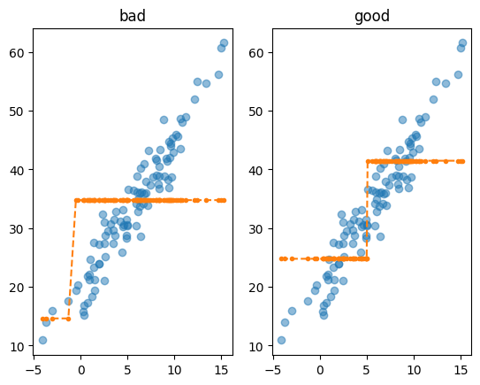

딱봐도 오른쪽이 좋은 분할같은데, 컴퓨터한테 이걸 어떻게 설명하지?

- 좋은분할을 구하는 이유는 좋은 yhat을 얻기 위함이다. 그렇다면 좋은 yhat을 얻게 해주는 분할이 좋은 분할이라 해석할 수 있다. \(\to\) 아이디어: 그런데 좋은 yhat은 sklearn.metrics.r2_score(y,yhat)의 값이 높지 않을까?

- 그렇다면 위의 그림에서 왼쪽보다 오른쪽이더 좋은 분할이라면 r2_score(y,yhat_good)의 값이 r2_score(y,yhat_bad) 값보다 높을 것!

sklearn.metrics.r2_score(y,yhat_bad), sklearn.metrics.r2_score(y,yhat_good)

(0.13932141536746745, 0.6167038863844928)

- 트리의 max_depth=1 일 경우 분할을 결정하는 방법 – 노가다..

적당한 \(c\)를 고른다.
분할 \((-\infty,c), [c,\infty)\) 를 생성하고 yhat를 계산한다.
r2_score(y,yhat)를 계산하고 기록한다.
1-3의 과정을 무한반복 한다. 그리고 r2_score(y,yhat)의 값을 가장 작게 만드는 \(c\)가 무엇인지 찾는다.

cuts = np.arange(-5,15)
fig = plt.figure()
def func(frame):
    ax = fig.gca()
    ax.clear()
    ax.plot(X,y,'o',alpha=0.5)
    c = cuts[frame] 
    yhat = fit_predict(X,y,c)
    ax.plot(X,yhat,'.')
    r2 = sklearn.metrics.r2_score(y,yhat)
    ax.set_title(f'c={c}, r2_score={r2:.2f}')

<Figure size 640x480 with 0 Axes>

ani = matplotlib.animation.FuncAnimation(
    fig,
    func,
    frames=20
)
display(IPython.display.HTML(ani.to_jshtml()))

- tree가 찾은 값 5.05를 우리가 직접 찾아보자.

cuts = np.arange(-5,15,0.05).round(2)
score = np.array([sklearn.metrics.r2_score(y,fit_predict(X,y,c)) for c in cuts])
plt.plot(cuts,score)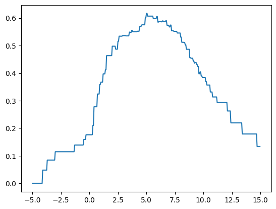

- 방법1: 시각화로 찾는방법

pd.DataFrame({'cut':cuts,'score':score})\
.plot.line(x='cut',y='score',backend='plotly')

- 방법2: 정석

cuts[score.argmax()]

5.0

- max_depth=2일 경우? max_depth=1의 결과로 발생한 2개의 조각을 각각 전체자료로 생각하고, max_depth=1일 때의 분할방법을 반복적용한다.

- X=[temp,type] 와 같은 경우라면? 설명변수를 하나씩 고정하여 각각 최적분할을 생성하고 r2_score관점에서 가장 우수한 설명변수를 선택

## step1
X = df_train[['temp']]
y = df_train['sales']
## step2
predictr = sklearn.tree.DecisionTreeRegressor(max_depth=2) 
## step3 
predictr.fit(X,y) 
## step4 -- pass 
# predictr.predict(X)

DecisionTreeRegressor(max_depth=2)

sklearn.tree.plot_tree(predictr)

[Text(0.5, 0.8333333333333334, 'x[0] <= 5.05\nsquared_error = 111.946\nsamples = 100\nvalue = 33.973'),
 Text(0.25, 0.5, 'x[0] <= 1.75\nsquared_error = 34.94\nsamples = 45\nvalue = 24.788'),
 Text(0.125, 0.16666666666666666, 'squared_error = 15.12\nsamples = 19\nvalue = 19.105'),
 Text(0.375, 0.16666666666666666, 'squared_error = 8.587\nsamples = 26\nvalue = 28.94'),
 Text(0.75, 0.5, 'x[0] <= 10.7\nsquared_error = 49.428\nsamples = 55\nvalue = 41.489'),
 Text(0.625, 0.16666666666666666, 'squared_error = 19.819\nsamples = 47\nvalue = 39.251'),
 Text(0.875, 0.16666666666666666, 'squared_error = 21.051\nsamples = 8\nvalue = 54.638')]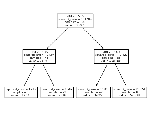

predictr.score(X,y)

0.8561424389856722

y_hat = y_pred = predictr.predict(X)
sklearn.metrics.r2_score(y,y_pred)

0.8561424389856722

yhat = ([y.mean()] * len(y))
r = y - yhat

sklearn.metrics.r2_score(y,r)

-9.31028261364953

df_train[df_train.temp<= 5.05].sales.mean(),df_train[df_train.temp> 5.05].sales.mean()

(24.787609205775055, 41.489079055828356)

df_a = df_train[df_train.temp<5.05]
X = df_a[['temp']]
y = df_a['sales']

cuts = np.arange(-5,15,0.05).round(2)
score = np.array([sklearn.metrics.r2_score(y,fit_predict(X,y,c)) for c in cuts])
plt.plot(cuts,score)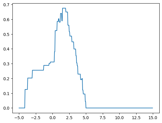

cuts[score.argmax()]

1.5

set(fit_predict(X,y,c=1.5))

{19.10544721087449, 28.939958355894696}

df_b = df_train[df_train.temp>=5.05]
X = df_b[['temp']]
y = df_b['sales']

cuts = np.arange(-5,15,0.05).round(2)
score = np.array([sklearn.metrics.r2_score(y,fit_predict(X,y,c)) for c in cuts])
plt.plot(cuts,score)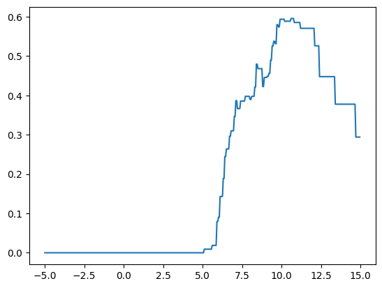

cuts[score.argmax()]

10.6

set(fit_predict(X,y,c=10.6))

{39.2509047276977, 54.63835323359588}

def fit_predict(X,y,c):
    X = np.array(X).reshape(-1)
    y = np.array(y) 
    yhat = y*0   
    yhat[X<=c] = y[X<=c].mean()
    yhat[X>c] = y[X>c].mean()
    return yhat

yhat_a = [y[X['weight'] < 43].mean()]
yhat_b = [y[(X['weight'] >=43) &  (X['weight'] < 56.33)].mean()]
yhat_c = [y[X['weight'] >= 56.33].mean()]
yhat = np.where(X['weight'] < 43, yhat_a, np.where((X['weight'] >= 43) & (X['weight'] < 56.33), yhat_b, yhat_c))

set(fit_predict(X,y,c=5.05))

{24.787609205775055, 41.489079055828356}