import numpy as np
import pandas as pd
import matplotlib.pyplot as plt
import seaborn as sns
import sklearn.metrics15wk-fin
최규빈
2023-12-21
- 의사결정나무의 수동구현은 위에서 제시된 모듈 (numpy, pandas, sklearn.metrics, matplotlib, seaborn) 만을 사용해야하며 이외의 모듈을 사용할 경우 0점 처리함.
- True/False를 판단하는 문제는 답만 써도 무방함. (이유를 써도 상관없음)
- Treu/False의 판단 문제는 모두 맞출 경우만 정답으로 인정함. 다만 틀린이유가 사소하다고 판단할경우 감점없이 만점처리함.
1. 의사결정나무의 수동구현 (70점)
df_train = pd.read_csv('https://raw.githubusercontent.com/guebin/MP2023/master/posts/height_train.csv')
df_train| weight | sex | height | |
|---|---|---|---|
| 0 | NaN | male | 164.227738 |
| 1 | NaN | male | 165.798660 |
| 2 | 75.219015 | male | 165.528672 |
| 3 | NaN | male | 163.706442 |
| 4 | 81.476750 | male | 165.501403 |
| ... | ... | ... | ... |
| 275 | 49.308558 | female | 148.587771 |
| 276 | NaN | male | 164.822474 |
| 277 | NaN | male | 163.907671 |
| 278 | NaN | male | 161.674476 |
| 279 | 53.714772 | female | 146.775975 |
280 rows × 3 columns
sns.lineplot(df_train, x = df_train['weight'], y = df_train['height'], hue=df_train['sex'])<AxesSubplot: xlabel='weight', ylabel='height'>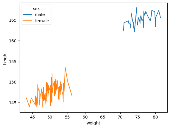
df_train.groupby('sex').describe()| weight | height | |||||||||||||||
|---|---|---|---|---|---|---|---|---|---|---|---|---|---|---|---|---|
| count | mean | std | min | 25% | 50% | 75% | max | count | mean | std | min | 25% | 50% | 75% | max | |
| sex | ||||||||||||||||
| female | 111.0 | 49.654963 | 2.503931 | 43.284661 | 47.833473 | 49.445699 | 51.400057 | 56.296321 | 111.0 | 147.436329 | 1.845190 | 143.832614 | 146.100147 | 147.605085 | 148.608729 | 153.475721 |
| male | 40.0 | 75.798872 | 2.685880 | 70.921502 | 73.758620 | 75.669420 | 77.294825 | 81.476750 | 169.0 | 164.915949 | 1.485475 | 160.195950 | 163.970895 | 164.947278 | 165.944777 | 169.223700 |
df_train['weight'].mean()56.580501947309074(1) df_train에서 “sex”,“weight”를 설명변수로 “height”을 반응변수로 설정하라. 결측치가 있을 경우 결측값에 일괄적으로 -99로 채워넣어라.
힌트: 결측치를 처리하기 위해 아래의 코드를 관찰하라.
df_toy = pd.DataFrame({'X':[1,2,np.nan,np.nan,5],'y':[3,4,5,1,2]})
df_toy| X | y | |
|---|---|---|
| 0 | 1.0 | 3 |
| 1 | 2.0 | 4 |
| 2 | NaN | 5 |
| 3 | NaN | 1 |
| 4 | 5.0 | 2 |
df_toy.fillna(-99)| X | y | |
|---|---|---|
| 0 | 1.0 | 3 |
| 1 | 2.0 | 4 |
| 2 | -99.0 | 5 |
| 3 | -99.0 | 1 |
| 4 | 5.0 | 2 |
df_tr = df_train.copy()
df_tr.info()
<class 'pandas.core.frame.DataFrame'>
RangeIndex: 280 entries, 0 to 279
Data columns (total 3 columns):
# Column Non-Null Count Dtype
--- ------ -------------- -----
0 weight 151 non-null float64
1 sex 280 non-null object
2 height 280 non-null float64
dtypes: float64(2), object(1)
memory usage: 6.7+ KBdf_train[df_train['sex'].isin(['female', 'male']) & df_train['weight'].isna()].groupby('sex').size()sex
male 129
dtype: int64- weight에 129개의 결측치가 있고, 다 남자이다.
df_tr = df_tr.fillna(-99)
df_tr.info()
<class 'pandas.core.frame.DataFrame'>
RangeIndex: 280 entries, 0 to 279
Data columns (total 3 columns):
# Column Non-Null Count Dtype
--- ------ -------------- -----
0 weight 280 non-null float64
1 sex 280 non-null object
2 height 280 non-null float64
dtypes: float64(2), object(1)
memory usage: 6.7+ KBX = df_tr[['sex','weight']]y = df_tr['height']X.head()| sex | weight | |
|---|---|---|
| 0 | male | -99.000000 |
| 1 | male | -99.000000 |
| 2 | male | 75.219015 |
| 3 | male | -99.000000 |
| 4 | male | 81.476750 |
y.head()0 164.227738
1 165.798660
2 165.528672
3 163.706442
4 165.501403
Name: height, dtype: float64(2) height열의 평균으로 height의 값을 추정하라. 추정값을 yhat에 저장하라. sklearn.metrics.r2_score()을 이용하여 r2_score를 계산하라.
hint: 0이 나와야 한다.
yhat = ([y.mean()] * len(y))
r2_score = sklearn.metrics.r2_score(y,yhat)
r2_score0.0(3) 아래를 계산하라.
r=y-yhat
여기에서 yhat은 (2)의 결과로 얻어진 적합값을 의미한다. 이제 r에 Weight를 기준으로 의사결정나무를 적용하여 아래와 같은 분할을 만들어라.
X['weight']<cX['weight']>=c
sklearn.metrics.r2_score()를 이용하여 최적의 \(c\)값을 구하여라.
참고
아래의 구간을 적당히 등분하여 구할 것. 너무 세밀하게 등분하지 않아도 무방함.
(X['weight'].min(), X['weight'].max())r = y - yhat
df_tr['r'] = rdef fit_predict(X,r,c):
X = np.array(X).reshape(-1)
r = np.array(r)
rhat = r*0
rhat[X<c] = r[X<c].mean()
rhat[X>=c] = r[X>=c].mean()
return rhatdef fit_predict_r(X,r,c):
X = np.array(X).reshape(-1)
r = np.array(r)
rhat = r*0
rhat[X<c] = r[X<c].mean()
rhat[X>=c] = r[X>=c].mean()
return rhatcuts = np.arange(X['weight'].min(), X['weight'].max(), 1)
score = np.array([sklearn.metrics.r2_score(r,fit_predict_r(X['weight'],r,c)) for c in cuts])/tmp/ipykernel_2473192/3973455866.py:5: RuntimeWarning: Mean of empty slice.
rhat[X<c] = r[X<c].mean()
/home/coco/anaconda3/envs/py38/lib/python3.8/site-packages/numpy/core/_methods.py:189: RuntimeWarning: invalid value encountered in double_scalars
ret = ret.dtype.type(ret / rcount)pd.DataFrame({'cut':cuts,'score':score})\
.plot.line(x='cut',y='score',backend='plotly')score.max()0.5320524394291484cuts[score == 0.5320524394291484]array([-98., -97., -96., -95., -94., -93., -92., -91., -90., -89., -88.,
-87., -86., -85., -84., -83., -82., -81., -80., -79., -78., -77.,
-76., -75., -74., -73., -72., -71., -70., -69., -68., -67., -66.,
-65., -64., -63., -62., -61., -60., -59., -58., -57., -56., -55.,
-54., -53., -52., -51., -50., -49., -48., -47., -46., -45., -44.,
-43., -42., -41., -40., -39., -38., -37., -36., -35., -34., -33.,
-32., -31., -30., -29., -28., -27., -26., -25., -24., -23., -22.,
-21., -20., -19., -18., -17., -16., -15., -14., -13., -12., -11.,
-10., -9., -8., -7., -6., -5., -4., -3., -2., -1., 0.,
1., 2., 3., 4., 5., 6., 7., 8., 9., 10., 11.,
12., 13., 14., 15., 16., 17., 18., 19., 20., 21., 22.,
23., 24., 25., 26., 27., 28., 29., 30., 31., 32., 33.,
34., 35., 36., 37., 38., 39., 40., 41., 42., 43.])c = 43 ~ -98일 때 score값이 제일 높다. 결측값(-99)의 영향으로 -99~43까지의 score값이 동일하다. 43을 기준으로 분할하겠다.
y했을때
def fit_predict(X,y,c):
    X = np.array(X['weight']).reshape(-1)
    y = np.array(y)
    yhat = y*0
    yhat[X<c] = y[X<c].mean()
    yhat[X>=c] = y[X>=c].mean()
    return yhat
cuts = np.arange(X['weight'].min(), X['weight'].max(), 1)
score = np.array([sklearn.metrics.r2_score(y,fit_predict(X,y,c)) for c in cuts])/tmp/ipykernel_1931661/1408215283.py:5: RuntimeWarning: Mean of empty slice.
yhat[X<c] = y[X<c].mean()
/home/coco/anaconda3/envs/py38/lib/python3.8/site-packages/numpy/core/_methods.py:189: RuntimeWarning: invalid value encountered in double_scalars
ret = ret.dtype.type(ret / rcount)pd.DataFrame({'cut':cuts,'score':score})\
.plot.line(x='cut',y='score',backend='plotly')sklearn.metrics.r2_score()을 이용하여 score값이 제일 큰 값 중, c = 43을 선택하겠다. 결측값(-99)의 영향으로 -99~43까지의 score값이 동일하다.
y[X['weight'] < 57].mean(),y[X['weight']>=57].mean()(156.7993284577238, 165.10972708769765)y[X['weight'] < 43].mean(),y[X['weight']>=43].mean()(164.85586311410242, 152.1180236532609)r[X['weight'] < 57].mean(),r[X['weight']>=57].mean()(-2.1652839057394444, 12.991703434436749)(4) (3)의 결과로 얻어진 아래의 분할을 고려하자.
X['weight'] >= c이 분할에서 depth=2 로 나무를 성장하고자 한다. 성장이가능한가? 성장이 가능하다면 이때 나무를 성장시키기 위한 변수로 weigth와 sex중 무엇이 적절한가? 왜 그렇다고 생각하는가?
X['weight'] >= 43분할 후 나무를 성장시킬 때 성장 변수로는 weight와 sex 중 어느 값을 선택해도 된다.X['weight'] >= 43데이터는 총 151개이다. 이 중 성별은 여성:남성 = 0.73:0.26의 비율을 가지고 남성체중의 min값이 여성 체중 max값보다 크다. 즉 해당 데이터에서는 어느 변수로 해도 동일한 값을 가질 것이다..
a = df_tr[df_tr['weight'] >=43]
a.groupby('sex')['height'].describe()| count | mean | std | min | 25% | 50% | 75% | max | |
|---|---|---|---|---|---|---|---|---|
| sex | ||||||||
| female | 111.0 | 147.436329 | 1.845190 | 143.832614 | 146.100147 | 147.605085 | 148.608729 | 153.475721 |
| male | 40.0 | 165.109727 | 1.481017 | 162.097926 | 164.176711 | 164.944052 | 166.185251 | 167.937239 |
X['weight'][X['weight'] >= 43].describe()count 151.000000
mean 56.580502
std 11.851509
min 43.284661
25% 48.510083
50% 50.675306
75% 71.704120
max 81.476750
Name: weight, dtype: float64X[X['weight'] >= 43].groupby('sex').describe()| weight | ||||||||
|---|---|---|---|---|---|---|---|---|
| count | mean | std | min | 25% | 50% | 75% | max | |
| sex | ||||||||
| female | 111.0 | 49.654963 | 2.503931 | 43.284661 | 47.833473 | 49.445699 | 51.400057 | 56.296321 |
| male | 40.0 | 75.798872 | 2.685880 | 70.921502 | 73.758620 | 75.669420 | 77.294825 | 81.476750 |
(5) (3)의 결과로 얻어진 아래의 분할을 고려하자.
X['weight'] < c이 분할에서 depth=2 로 나무를 성장하고자 한다. 성장이가능한가? 성장이 가능하다면 이때 나무를 성장시키기 위한 변수로 weigth와 sex중 무엇이 적절한가? 왜 그렇다고 생각하는가?
(X['weight']==-99).sum()129129/2800.4607142857142857- 성장이 가능하지 않다. NaN(-99대치)값으로 인해서 rscore의 값이 제일 큰 c값을 결정했다. 해당 데이터에서 결측치는 46%를 차지한다. 처음 분할에서 정한 c값보다 작은 weight의 값은 모두 결측치이다. 그러므로 더 이상 성장할 수 없다.
(6) (3)-(5)의 결과를 이용하여 depth=2인 의사결정나무에 의한 r의 적합값을 구하여라. 이를 이용하여 yhat을 update하라. 이때 학습률은 0.1로 설정하고 업데이트된 결과를 yhat2로 저장하라. 그리고sklearn.metrics.r2_score()을 이용하여 y와 yhat2의 r2_score를 계산하라.
힌트: 아래의 알고리즘이 동치임을 이용하라.
yhat2\(\leftarrow\)yhat+ 학습률 \(\times\)rhatr2\(\leftarrow\)r- 학습률 \(\times\)rhat, wherer2=y-yhat2
- depth=2에서의 분할값의 기준인 c2값찾기(초반 r = y-yhat은 (3)에서 적합한 값으로 계산하였음..)
df_tr2 = df_tr[df_tr['weight'] >= 43]cuts2 = np.arange(df_tr2['weight'].min(), df_tr2['weight'].max(), 1)
score2 = np.array([sklearn.metrics.r2_score(df_tr2['r'],fit_predict_r(df_tr2['weight'],df_tr2['r'],c)) for c in cuts2])/tmp/ipykernel_2473192/3973455866.py:5: RuntimeWarning:
Mean of empty slice.
/home/coco/anaconda3/envs/py38/lib/python3.8/site-packages/numpy/core/_methods.py:189: RuntimeWarning:
invalid value encountered in double_scalars
pd.DataFrame({'cut':cuts2,'score':score2})\
.plot.line(x='cut',y='score',backend='plotly')score2.max()0.9522972193365125- 두 번째에서는 c=64값을 선택하겠다.
_, a = set(fit_predict_r(X['weight'],r,c=43))b, c = set(fit_predict_r(df_tr2['weight'],df_tr2['r'],c=64))- r의 적합값: r2
(1) X['weight'] < 43   -> r2 = 6.86933485209669    : a

(2) 43 =< X['weight'] < 64   -> r2 = -10.550199540073395 : b

(3) X['weight'] >=64 -> r2 = 7.123198825691906 : cdf_tr.loc[df_tr['weight'] < 43, 'r2'] = a
df_tr.loc[(df_tr['weight'] >= 43) & (df_tr['weight'] < 64),'r2'] = b
df_tr.loc[df_tr['weight'] >= 64, 'r2'] = cyhat = y - df_tr['r2']rhat = (df_tr['r'] - df_tr['r2'])*10yhat2 = yhat + 0.1 * rhatsklearn.metrics.r2_score(y,yhat2)-4.218847493575595e-15y.mean()157.98652826200575yhat2.mean()157.98652826200575r = y-yhat
y
- (1) 경우
yhat_a = ([y[X['weight'] < 43].mean()] * len(y[X['weight'] < 43]))
yhat_b = ([y[X['weight'] >=43].mean()] * len(y[X['weight'] >=43]))sklearn.metrics.r2_score(y,yhat)0.5320524394291483r = y - yhatr_a = [r[X['weight'] < 43].mean()]
r_b = [r[(X['weight'] >=43) & (X['weight'] < 56.33)].mean()]
r_c = [r[X['weight'] >= 56.33].mean()]
rhat = np.where(X['weight'] < 43, r_a, np.where((X['weight'] >= 43) & (X['weight'] < 56.33), r_b, r_c))yhat_a = [y[X['weight'] < 43].mean()]
yhat_b = [y[(X['weight'] >=43) & (X['weight'] < 56.33)].mean()]
yhat_c = [y[X['weight'] >= 56.33].mean()]
yhat23 = np.where(X['weight'] < 43, yhat_a, np.where((X['weight'] >= 43) & (X['weight'] < 56.33), yhat_b, yhat_c))r = y - yhat- (2) 경우
- 방법1(위에서 찾은 그 다음 구간의 score값이 제일 높은 c값을 찾아줌..)
yhat_c = [y[(X['weight'] >=43) &  (X['weight'] < 56.33)].mean()]
yhat_d = [y[X['weight'] >= 56.33].mean()]
yhat2 = np.where(X['weight'] < 43, yhat_a, np.where((X['weight'] >= 43) & (X['weight'] < 56.33), yhat_c, yhat_d))sklearn.metrics.r2_score(y,yhat2)0.9649652393240589- 방법2(알고리즘 사용)
r2 = y-yhat2yhat_2 = yhat + 0.1*r2yhat_20 164.793051
1 164.950143
2 152.159918
3 164.740921
4 152.157191
...
275 152.233168
276 164.852524
277 164.761044
278 164.537724
279 152.051988
Name: height, Length: 280, dtype: float64sklearn.metrics.r2_score(y,yhat_2)0.5387090439575772r2NameError: name 'r2' is not defined(7) (6)에서 학습률이 0.5일 경우 y와 yhat2의 r2_score를 계산하라.
yhat3 = yhat + 0.5 * rhatsklearn.metrics.r2_score(y,yhat3)-0.8408342562225903yhat3.mean()157.986528262005752. 다음을 읽고 참거짓을 판단하라. (30점)
(1) 의사결정나무에서 max_depth의 설정값이 커질수록 오버피팅의 위험이 있다.
T
(2) 배깅의 설명변수중 일부를 drop 하며 나무를 성장시킨다.
F (배깅은 가지치기가 필요없당)
(3) 랜덤포레스트는 나무가지를 랜덤으로 성장시키기도 하고 파괴시키기도 한다.
F (가지치기에 대한 설명 같은데, 의사결정나무가 해당된다..)
(4) 부스팅은 여러가지 의사결정나무의 적합값을 평균내는 방식으로 최종예측을 한다.
F (배깅에 대한 설명)
(5) Accuracy는 분류문제에서 언제나 가장 합리적인 평가지표이다.
F
(6) 모듈49의 아래그림은 “sex == ‘male’” 일 경우 “sex=‘female’” 일때보다 항상(=모든 관측치에 대하여) 키의 예측값을 +2.1 만큼 보정해야 한다는 것을 의미한다.
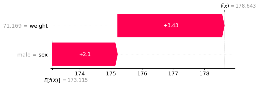
F
(7) 모듈54에서 제시된 아래의 그림은 사실 전혀 고려할 필요가 없다.
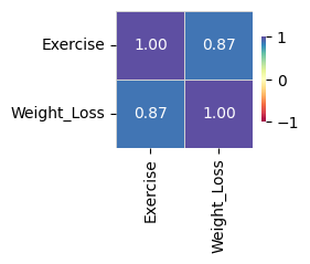
왜냐하면 Exercise는 범주형, Weight_Loss는 연속형이므로 correlation값은 의미가 없기 때문이다.
F
(8) 시계열분석에서 static_feature란 이미 알고있는 미래의 시계열자료를 의미한다.
F
(9) 모듈59에서 소개된 자전거대여자료와 같이 시간특징이 포함된 자료는 언제나 (과거를 기반으로 미래를 예측하는) 시계열분석을 하는 것이 올바르다.
F
(10) 모듈60에서 소개된 하이퍼파라메터 설정법을 이용하면 때때로 모형의 적합도를 높일 수 있다.
T