import networkx as nx
import matplotlib.pyplot as plt
G=nx.Graph()
V={'D','P','M','R'}
E=[('M','A'),('M','P'),('P','D'),('M','R')]
G.add_nodes_from(V)
G.add_edges_from(E)ref
단순무향그래프 \(G=(V,E)\)
노드(꼭지점)의 집합: \(V=\{v_1,\dots,v_n\}\)
두 노도 간의 연결 나타내는 간선(변): \(E=\{(v_k,v_w),\dots,(v_i,v_j)\}\)
\(E\)의 각 원소는 순서쌍이며 각 간선 간에는 순서가 없다. \(\to (v_k,v_w) = (v_w,v_k)\)
\(|V|\):그래프의 위수(order)
\(|E|\): 그래프의 크기(size)
노드의 차수(degree): 해당 노드에 연결된 간선의 개수
\(v\)의 근방(neighbor): \(v\)에 연결된 모든 노드 \(V\)의 부분집합
print(f"V={G.nodes}")
print(f"E={G.edges}")
V=['M', 'R', 'P', 'D', 'A']
E=[('M', 'A'), ('M', 'P'), ('M', 'R'), ('P', 'D')]{G.degree(v): v for v in G.nodes}{3: 'M', 1: 'A', 2: 'P'}print(f"Graph Order위수: {G.number_of_nodes()}")
print(f"Graph Size크기: {G.number_of_edges()}")
print(f"Degree for nodes노드의 차수: { {v: G.degree(v) for v in G.nodes} }")
print(f"Neighbors for nodes근방노드: { {v: list(G.neighbors(v)) for v in G.nodes} }")Graph Order위수: 5
Graph Size크기: 4
Degree for nodes노드의 차수: {'M': 3, 'R': 1, 'P': 2, 'D': 1, 'A': 1}
Neighbors for nodes근방노드: {'M': ['A', 'P', 'R'], 'R': ['M'], 'P': ['M', 'D'], 'D': ['P'], 'A': ['M']}ego_graph_milan = nx.ego_graph(G, "M")
print(f"Nodes: {ego_graph_milan.nodes}")
print(f"Edges: {ego_graph_milan.edges}")Nodes: ['M', 'R', 'P', 'A']
Edges: [('M', 'A'), ('M', 'P'), ('M', 'R')]# 새로운 노드나 간선 추가
new_nodes = {'L', 'M'}
new_edges = [('L','R'), ('M','P')]
G.add_nodes_from(new_nodes)
G.add_edges_from(new_edges)
print(f"V = {G.nodes}")
print(f"E = {G.edges}")V = ['M', 'R', 'P', 'D', 'A', 'L']
E = [('M', 'A'), ('M', 'P'), ('M', 'R'), ('R', 'L'), ('P', 'D')]# 노드 삭제
node_remove = {'L', 'M'}
G.remove_nodes_from(node_remove)
print(f"V = {G.nodes}")
print(f"E = {G.edges}")V = ['R', 'P', 'D', 'A']
E = [('P', 'D')]# 간선 삭제
node_edges = [('M','D'), ('M','P')]
G.remove_edges_from(node_edges)
print(f"V = {G.nodes}")
print(f"E = {G.edges}")V = ['R', 'P', 'D', 'A']
E = [('P', 'D')]print(nx.to_edgelist(G))
print(nx.to_pandas_adjacency(G))[('P', 'D', {})]
R P D A
R 0.0 0.0 0.0 0.0
P 0.0 0.0 1.0 0.0
D 0.0 1.0 0.0 0.0
A 0.0 0.0 0.0 0.0유향그래프 \(G=(V,E)\)
노드(꼭지점)의 집합: \(V=\{v_1,\dots,v_n\}\)
두 노도 간의 연결 나타내는 간선(변): \(E=\{(v_k,v_w),\dots,(v_i,v_j)\}\)
\(E\)의 각 원소는 순서쌍이며 각 간선 간에는 순서가 있다. \(\to (v_k,v_w) \neq (v_w,v_k)\)
입력차수(indegree) \(deg^-(v)\) : 노드 \(v\)로 도착하는 간선의 개수
출력차수(outdegree) \(deg^+(v)\): 노드 \(v\)에서 출발하는 간선의 개수
다중그래프 \(G=(V,E)\)
한 노드에서 출발해서 같은 노드로 도착하는 간선이 여러 개인 다중 간선이 있는 그래프
\(V\): 노드의 집합, \(E\): 간선의 다중집합
유향다중그래프: 순서쌍의 다중집합
무향다중그래프: 순서가 없는 경우
가중그래프
간선가중그래프 \(G=(V,E,w)\)
- \(V\): 노드의 집합, \(E\): 간선의 집합, \(w: E \to \mathbb{R}\): 각 간선을 실수 \(e \in E\) 가중값으로 대중시키는 가중함수
노드가중그래프 \(G=(V,E,w)\)
- \(V\): 노드의 집합, \(E\): 간선의 집합, \(w: V \to \mathbb{R}\): 각 간선을 실수 \(v \in V\) 가중값으로 대중시키는 가중함수
다분그래프(k분그래프)
- 노드를 각각 2개, 3개, k개의 노드 집합으로 분할할 수 있음
그래프신호 기본
import matplotlib.pyplot as plt
import numpy as np

# x축 값 생성
x = np.arange(0, 10, 0.1)

# y축 값 생성
y = np.sin(x)

# 그래프 그리기
plt.plot(x, y)
plt.xlabel('x')
plt.ylabel('y')
plt.title('Sine Wave')
plt.show()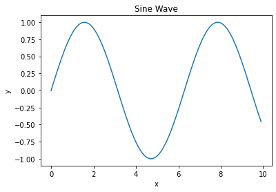
그래프 클러스터링 기본
import networkx as nx
import matplotlib.pyplot as plt

# 그래프 생성
G = nx.karate_club_graph()

# 클러스터링 수행
clusters = nx.algorithms.community.greedy_modularity_communities(G)

# 클러스터링 결과 출력
for i, c in enumerate(clusters):
    print(f"Cluster {i}: {c}")
    nx.draw_networkx_nodes(G, pos=nx.spring_layout(G), nodelist=list(c), node_color=[i]*len(c), cmap=plt.cm.tab20, node_size=200)

nx.draw_networkx_edges(G, pos=nx.spring_layout(G), alpha=0.5)
plt.axis("off")
plt.show()
Cluster 0: frozenset({8, 14, 15, 18, 20, 22, 23, 24, 25, 26, 27, 28, 29, 30, 31, 32, 33})
Cluster 1: frozenset({1, 2, 3, 7, 9, 12, 13, 17, 21})
Cluster 2: frozenset({0, 16, 19, 4, 5, 6, 10, 11})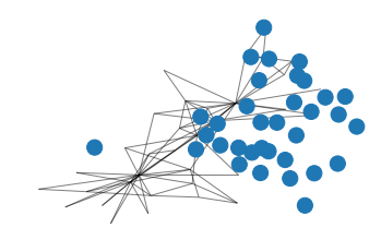
- 그래프 클러스터링 논문
- Newman, M. E. J., & Girvan, M. (2004). Finding and evaluating community structure in networks. Physical Review E, 69(2), 026113. - 그래프의 모듈러리티(Modularity)를 최대화하는 방식으로 클러스터링을 수행 - Girvan-Newman 알고리즘
- Blondel, V. D., Guillaume, J.-L., Lambiotte, R., & Lefebvre, E. (2008). Fast unfolding of communities in large networks. Journal of Statistical Mechanics: Theory and Experiment, 2008(10), P10008. - 그래프를 분할하는 방식으로 클러스터링을 수행
- Leskovec, J., Lang, K. J., & Mahoney, M. W. (2010). Empirical comparison of algorithms for network community detection. Proceedings of the 19th international conference on World wide web, 631-640. - 여러 그래프 클러스터링 알고리즘을 비교하는 실험을 수행 - 그래프의 크기, 밀도, 구조 등에 따라 다양한 알고리즘이 잘 작동
- Fortunato, S., & Hric, D. (2016). Community detection in networks: A user guide. Physics Reports, 659, 1-44. - 그래프 클러스터링의 기본 개념과 다양한 알고리즘을 상세히 설명하고, 이를 이용하여 실제 그래프에서의 클러스터링을 수행하는 방법을 제시
예제(k-means)
from sklearn.cluster import KMeans
from sklearn.datasets import load_iris
import pandas as pd
import matplotlib.pyplot as plt
# 데이터셋 로드
iris = load_iris()
df = pd.DataFrame(data=iris.data, columns=iris.feature_names)# 모델 생성 및 학습
kmeans = KMeans(n_clusters=3, random_state=0)
kmeans.fit(df)/home/coco/anaconda3/envs/py38/lib/python3.8/site-packages/sklearn/cluster/_kmeans.py:870: FutureWarning: The default value of `n_init` will change from 10 to 'auto' in 1.4. Set the value of `n_init` explicitly to suppress the warning
warnings.warn(KMeans(n_clusters=3, random_state=0)In a Jupyter environment, please rerun this cell to show the HTML representation or trust the notebook.
On GitHub, the HTML representation is unable to render, please try loading this page with nbviewer.org.
KMeans(n_clusters=3, random_state=0)
# 클러스터링 결과 시각화
df['cluster'] = kmeans.labels_
plt.scatter(df['petal length (cm)'], df['petal width (cm)'], c=df['cluster'])
plt.xlabel('petal length (cm)')
plt.ylabel('petal width (cm)')
plt.show()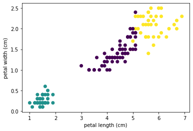
- ref: [출처] 클러스터링(Clustering)이란? 클러스터링 특징, 종류, 예제 실습|작성자 리르시