dt <- data.frame(
  x1 = c(7,1,11,11,7,11,3,1,2,21,1,11,10),
  x2 = c(26,29,56,31,52,55,71,31,54,47,40,66,68),
  x3 = c(6,15,8,8,6,9,17,22,18,4,23,9,8),
  x4 = c(60,52,20,47,33,22,6,44,22,26,34,12,12),
  y  = c(78.5,74.3,104.3,87.6,95.9,109.2,102.7,72.5,93.1,115.9,83.8,113.3,109.4)
)해당 강의노트는 전북대학교 이영미교수님 2022-2 고급회귀분석론 자료임
pairs(dt, pch=16)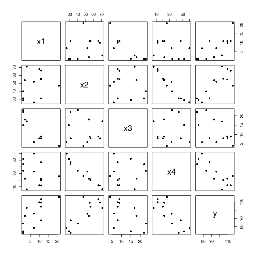
cor(dt)| x1 | x2 | x3 | x4 | y | |
|---|---|---|---|---|---|
| x1 | 1.0000000 | 0.2285795 | -0.8241338 | -0.2454451 | 0.7307175 |
| x2 | 0.2285795 | 1.0000000 | -0.1392424 | -0.9729550 | 0.8162526 |
| x3 | -0.8241338 | -0.1392424 | 1.0000000 | 0.0295370 | -0.5346707 |
| x4 | -0.2454451 | -0.9729550 | 0.0295370 | 1.0000000 | -0.8213050 |
| y | 0.7307175 | 0.8162526 | -0.5346707 | -0.8213050 | 1.0000000 |
m <- lm(y~., dt)  ##FM
summary(m)
Call:
lm(formula = y ~ ., data = dt)

Residuals:
    Min      1Q  Median      3Q     Max
-3.1750 -1.6709  0.2508  1.3783  3.9254

Coefficients:
            Estimate Std. Error t value Pr(>|t|)
(Intercept)  62.4054    70.0710   0.891   0.3991
x1            1.5511     0.7448   2.083   0.0708 .
x2            0.5102     0.7238   0.705   0.5009
x3            0.1019     0.7547   0.135   0.8959
x4           -0.1441     0.7091  -0.203   0.8441
---
Signif. codes:  0 ‘***’ 0.001 ‘**’ 0.01 ‘*’ 0.05 ‘.’ 0.1 ‘ ’ 1

Residual standard error: 2.446 on 8 degrees of freedom
Multiple R-squared:  0.9824,    Adjusted R-squared:  0.9736
F-statistic: 111.5 on 4 and 8 DF, p-value: 4.756e-07anova(m)| Df | Sum Sq | Mean Sq | F value | Pr(>F) | |
|---|---|---|---|---|---|
| <int> | <dbl> | <dbl> | <dbl> | <dbl> | |
| x1 | 1 | 1450.0763281 | 1450.0763281 | 242.36791816 | 2.887559e-07 |
| x2 | 1 | 1207.7822656 | 1207.7822656 | 201.87052753 | 5.863323e-07 |
| x3 | 1 | 9.7938691 | 9.7938691 | 1.63696188 | 2.366003e-01 |
| x4 | 1 | 0.2469747 | 0.2469747 | 0.04127972 | 8.440715e-01 |
| Residuals | 8 | 47.8636394 | 5.9829549 | NA | NA |
##### 후진제거법
summary(m) #x3 제거
# drop1(m, test = "F")
Call:
lm(formula = y ~ ., data = dt)

Residuals:
    Min      1Q  Median      3Q     Max
-3.1750 -1.6709  0.2508  1.3783  3.9254

Coefficients:
            Estimate Std. Error t value Pr(>|t|)
(Intercept)  62.4054    70.0710   0.891   0.3991
x1            1.5511     0.7448   2.083   0.0708 .
x2            0.5102     0.7238   0.705   0.5009
x3            0.1019     0.7547   0.135   0.8959
x4           -0.1441     0.7091  -0.203   0.8441
---
Signif. codes:  0 ‘***’ 0.001 ‘**’ 0.01 ‘*’ 0.05 ‘.’ 0.1 ‘ ’ 1

Residual standard error: 2.446 on 8 degrees of freedom
Multiple R-squared:  0.9824,    Adjusted R-squared:  0.9736
F-statistic: 111.5 on 4 and 8 DF,  p-value: 4.756e-07
m1 <- update(m, ~ . -x3)
summary(m1) #x4 제거
# drop1(m1, test = "F")
Call:
lm(formula = y ~ x1 + x2 + x4, data = dt)

Residuals:
    Min      1Q  Median      3Q     Max
-3.0919 -1.8016  0.2562  1.2818  3.8982

Coefficients:
            Estimate Std. Error t value Pr(>|t|)
(Intercept)  71.6483    14.1424   5.066 0.000675 ***
x1            1.4519     0.1170  12.410 5.78e-07 ***
x2            0.4161     0.1856   2.242 0.051687 .
x4           -0.2365     0.1733  -1.365 0.205395
---
Signif. codes:  0 ‘***’ 0.001 ‘**’ 0.01 ‘*’ 0.05 ‘.’ 0.1 ‘ ’ 1

Residual standard error: 2.309 on 9 degrees of freedom
Multiple R-squared:  0.9823,    Adjusted R-squared:  0.9764
F-statistic: 166.8 on 3 and 9 DF,  p-value: 3.323e-08
m2 <- update(m1, ~ . -x4)
summary(m2)  #x4 제거
# drop1(m2, test = "F")
Call:
lm(formula = y ~ x1 + x2, data = dt)

Residuals:
   Min     1Q Median     3Q    Max
-2.893 -1.574 -1.302  1.363  4.048

Coefficients:
            Estimate Std. Error t value Pr(>|t|)
(Intercept) 52.57735    2.28617   23.00 5.46e-10 ***
x1           1.46831    0.12130   12.11 2.69e-07 ***
x2           0.66225    0.04585   14.44 5.03e-08 ***
---
Signif. codes:  0 ‘***’ 0.001 ‘**’ 0.01 ‘*’ 0.05 ‘.’ 0.1 ‘ ’ 1

Residual standard error: 2.406 on 10 degrees of freedom
Multiple R-squared:  0.9787,    Adjusted R-squared:  0.9744
F-statistic: 229.5 on 2 and 10 DF,  p-value: 4.407e-09
##### 전진선택법
m0 = lm(y ~ 1, data = dt)
add1(m0,
     scope = y ~  x1 + x2 + x3+ x4,
test = "F") ## x4추가| Df | Sum of Sq | RSS | AIC | F value | Pr(>F) | |
|---|---|---|---|---|---|---|
| <dbl> | <dbl> | <dbl> | <dbl> | <dbl> | <dbl> | |
| <none> | NA | NA | 2715.7631 | 71.44443 | NA | NA |
| x1 | 1 | 1450.0763 | 1265.6867 | 63.51947 | 12.602518 | 0.0045520446 |
| x2 | 1 | 1809.4267 | 906.3363 | 59.17799 | 21.960605 | 0.0006648249 |
| x3 | 1 | 776.3626 | 1939.4005 | 69.06740 | 4.403417 | 0.0597623242 |
| x4 | 1 | 1831.8962 | 883.8669 | 58.85164 | 22.798520 | 0.0005762318 |
m1 <- update(m0, ~ . +x4)
summary(m1)
Call:
lm(formula = y ~ x4, data = dt)

Residuals:
    Min      1Q  Median      3Q     Max
-12.589  -8.228   1.495   4.726  17.524

Coefficients:
            Estimate Std. Error t value Pr(>|t|)
(Intercept) 117.5679     5.2622  22.342 1.62e-10 ***
x4           -0.7382     0.1546  -4.775 0.000576 ***
---
Signif. codes:  0 ‘***’ 0.001 ‘**’ 0.01 ‘*’ 0.05 ‘.’ 0.1 ‘ ’ 1

Residual standard error: 8.964 on 11 degrees of freedom
Multiple R-squared:  0.6745,    Adjusted R-squared:  0.645
F-statistic: 22.8 on 1 and 11 DF, p-value: 0.0005762add1(m1,
scope = y ~ x1 + x2 + x3+ x4,
test = "F") ## x1추가| Df | Sum of Sq | RSS | AIC | F value | Pr(>F) | |
|---|---|---|---|---|---|---|
| <dbl> | <dbl> | <dbl> | <dbl> | <dbl> | <dbl> | |
| <none> | NA | NA | 883.86692 | 58.85164 | NA | NA |
| x1 | 1 | 809.10480 | 74.76211 | 28.74170 | 108.2239093 | 1.105281e-06 |
| x2 | 1 | 14.98679 | 868.88013 | 60.62933 | 0.1724839 | 6.866842e-01 |
| x3 | 1 | 708.12891 | 175.73800 | 39.85258 | 40.2945802 | 8.375467e-05 |
m2 <- update(m1, ~ . +x1)
summary(m2)
Call:
lm(formula = y ~ x4 + x1, data = dt)

Residuals:
    Min      1Q  Median      3Q     Max
-5.0234 -1.4737  0.1371  1.7305  3.7701

Coefficients:
             Estimate Std. Error t value Pr(>|t|)
(Intercept) 103.09738    2.12398   48.54 3.32e-13 ***
x4           -0.61395    0.04864  -12.62 1.81e-07 ***
x1            1.43996    0.13842   10.40 1.11e-06 ***
---
Signif. codes:  0 ‘***’ 0.001 ‘**’ 0.01 ‘*’ 0.05 ‘.’ 0.1 ‘ ’ 1

Residual standard error: 2.734 on 10 degrees of freedom
Multiple R-squared:  0.9725,    Adjusted R-squared:  0.967
F-statistic: 176.6 on 2 and 10 DF, p-value: 1.581e-08add1(m2,
scope = y ~ x1 + x2 + x3+ x4,
test = "F") ## stop| Df | Sum of Sq | RSS | AIC | F value | Pr(>F) | |
|---|---|---|---|---|---|---|
| <dbl> | <dbl> | <dbl> | <dbl> | <dbl> | <dbl> | |
| <none> | NA | NA | 74.76211 | 28.74170 | NA | NA |
| x2 | 1 | 26.78938 | 47.97273 | 24.97388 | 5.025865 | 0.05168735 |
| x3 | 1 | 23.92599 | 50.83612 | 25.72755 | 4.235846 | 0.06969226 |
##### 단계적선택법
m0 = lm(y ~ 1, data = dt)
add1(m0,
     scope = y ~  x1 + x2 + x3+ x4,
     test = "F")  ## x4추가
m1 <- update(m0, ~ . +x4)| Df | Sum of Sq | RSS | AIC | F value | Pr(>F) | |
|---|---|---|---|---|---|---|
| <dbl> | <dbl> | <dbl> | <dbl> | <dbl> | <dbl> | |
| <none> | NA | NA | 2715.7631 | 71.44443 | NA | NA |
| x1 | 1 | 1450.0763 | 1265.6867 | 63.51947 | 12.602518 | 0.0045520446 |
| x2 | 1 | 1809.4267 | 906.3363 | 59.17799 | 21.960605 | 0.0006648249 |
| x3 | 1 | 776.3626 | 1939.4005 | 69.06740 | 4.403417 | 0.0597623242 |
| x4 | 1 | 1831.8962 | 883.8669 | 58.85164 | 22.798520 | 0.0005762318 |
m1 <- update(m0, ~ . +x4)
summary(m1)
Call:
lm(formula = y ~ x4, data = dt)

Residuals:
    Min      1Q  Median      3Q     Max
-12.589  -8.228   1.495   4.726  17.524

Coefficients:
            Estimate Std. Error t value Pr(>|t|)
(Intercept) 117.5679     5.2622  22.342 1.62e-10 ***
x4           -0.7382     0.1546  -4.775 0.000576 ***
---
Signif. codes:  0 ‘***’ 0.001 ‘**’ 0.01 ‘*’ 0.05 ‘.’ 0.1 ‘ ’ 1

Residual standard error: 8.964 on 11 degrees of freedom
Multiple R-squared:  0.6745,    Adjusted R-squared:  0.645
F-statistic: 22.8 on 1 and 11 DF, p-value: 0.0005762add1(m1,
scope = y ~ x1 + x2 + x3+ x4,
test = "F") ## x1추가
m2 <- update(m1, ~ . +x1)
summary(m2) #제거 없음| Df | Sum of Sq | RSS | AIC | F value | Pr(>F) | |
|---|---|---|---|---|---|---|
| <dbl> | <dbl> | <dbl> | <dbl> | <dbl> | <dbl> | |
| <none> | NA | NA | 883.86692 | 58.85164 | NA | NA |
| x1 | 1 | 809.10480 | 74.76211 | 28.74170 | 108.2239093 | 1.105281e-06 |
| x2 | 1 | 14.98679 | 868.88013 | 60.62933 | 0.1724839 | 6.866842e-01 |
| x3 | 1 | 708.12891 | 175.73800 | 39.85258 | 40.2945802 | 8.375467e-05 |
Call:
lm(formula = y ~ x4 + x1, data = dt)

Residuals:
    Min      1Q  Median      3Q     Max
-5.0234 -1.4737  0.1371  1.7305  3.7701

Coefficients:
             Estimate Std. Error t value Pr(>|t|)
(Intercept) 103.09738    2.12398   48.54 3.32e-13 ***
x4           -0.61395    0.04864  -12.62 1.81e-07 ***
x1            1.43996    0.13842   10.40 1.11e-06 ***
---
Signif. codes:  0 ‘***’ 0.001 ‘**’ 0.01 ‘*’ 0.05 ‘.’ 0.1 ‘ ’ 1

Residual standard error: 2.734 on 10 degrees of freedom
Multiple R-squared:  0.9725,    Adjusted R-squared:  0.967
F-statistic: 176.6 on 2 and 10 DF, p-value: 1.581e-08add1(m2,
scope = y ~ x1 + x2 + x3+ x4,
test = "F") ## x2추가
m3 <- update(m2, ~ . +x2)
summary(m3) #x4 제거| Df | Sum of Sq | RSS | AIC | F value | Pr(>F) | |
|---|---|---|---|---|---|---|
| <dbl> | <dbl> | <dbl> | <dbl> | <dbl> | <dbl> | |
| <none> | NA | NA | 74.76211 | 28.74170 | NA | NA |
| x2 | 1 | 26.78938 | 47.97273 | 24.97388 | 5.025865 | 0.05168735 |
| x3 | 1 | 23.92599 | 50.83612 | 25.72755 | 4.235846 | 0.06969226 |
Call:
lm(formula = y ~ x4 + x1 + x2, data = dt)

Residuals:
    Min      1Q  Median      3Q     Max
-3.0919 -1.8016  0.2562  1.2818  3.8982

Coefficients:
            Estimate Std. Error t value Pr(>|t|)
(Intercept)  71.6483    14.1424   5.066 0.000675 ***
x4           -0.2365     0.1733  -1.365 0.205395
x1            1.4519     0.1170  12.410 5.78e-07 ***
x2            0.4161     0.1856   2.242 0.051687 .
---
Signif. codes:  0 ‘***’ 0.001 ‘**’ 0.01 ‘*’ 0.05 ‘.’ 0.1 ‘ ’ 1

Residual standard error: 2.309 on 9 degrees of freedom
Multiple R-squared:  0.9823,    Adjusted R-squared:  0.9764
F-statistic: 166.8 on 3 and 9 DF,  p-value: 3.323e-08
m4 <- update(m3, ~ . -x4)
add1(m4,
scope = y ~ x1 + x2 + x3+ x4,
test = "F") #stop| Df | Sum of Sq | RSS | AIC | F value | Pr(>F) | |
|---|---|---|---|---|---|---|
| <dbl> | <dbl> | <dbl> | <dbl> | <dbl> | <dbl> | |
| <none> | NA | NA | 57.90448 | 25.41999 | NA | NA |
| x3 | 1 | 9.793869 | 48.11061 | 25.01120 | 1.832128 | 0.2088895 |
| x4 | 1 | 9.931754 | 47.97273 | 24.97388 | 1.863262 | 0.2053954 |
# install.packages("leaps")
library(leaps)fit<-regsubsets(y~., data=dt, nbest=1,nvmax=4,
# method=c("exhaustive","backward",
# "forward", "seqrep")
method='forward',
)a <- summary(fit)
str(a)List of 8
$ which : logi [1:4, 1:5] TRUE TRUE TRUE TRUE FALSE TRUE ...
..- attr(*, "dimnames")=List of 2
.. ..$ : chr [1:4] "1" "2" "3" "4"
.. ..$ : chr [1:5] "(Intercept)" "x1" "x2" "x3" ...
$ rsq : num [1:4] 0.675 0.972 0.982 0.982
$ rss : num [1:4] 883.9 74.8 48 47.9
$ adjr2 : num [1:4] 0.645 0.967 0.976 0.974
$ cp : num [1:4] 138.73 5.5 3.02 5
$ bic : num [1:4] -9.46 -39.01 -42.21 -39.68
$ outmat: chr [1:4, 1:4] " " "*" "*" "*" ...
..- attr(*, "dimnames")=List of 2
.. ..$ : chr [1:4] "1 ( 1 )" "2 ( 1 )" "3 ( 1 )" "4 ( 1 )"
.. ..$ : chr [1:4] "x1" "x2" "x3" "x4"
$ obj :List of 28
..$ np : int 5
..$ nrbar : int 10
..$ d : num [1:5] 13 3362 390.2 154.7 10.5
..$ rbar : num [1:10] 30 7.4615 48.1538 11.7692 -0.0863 ...
..$ thetab : num [1:5] 95.423 -0.738 1.44 0.416 0.102
..$ first : int 2
..$ last : int 5
..$ vorder : int [1:5] 1 5 2 3 4
..$ tol : num [1:5] 1.80e-09 9.67e-08 2.36e-08 1.19e-07 3.72e-08
..$ rss : num [1:5] 2715.8 883.9 74.8 48 47.9
..$ bound : num [1:5] 2715.8 1265.7 57.9 48.1 47.9
..$ nvmax : int 5
..$ ress : num [1:5, 1] 2715.8 883.9 74.8 48 47.9
..$ ir : int 5
..$ nbest : num 1
..$ lopt : int [1:15, 1] 1 1 5 1 5 2 1 5 2 3 ...
..$ il : int 15
..$ ier : int 0
..$ xnames : chr [1:5] "(Intercept)" "x1" "x2" "x3" ...
..$ method : chr "forward"
..$ force.in : Named logi [1:5] TRUE FALSE FALSE FALSE FALSE
.. ..- attr(*, "names")= chr [1:5] "" "x1" "x2" "x3" ...
..$ force.out: Named logi [1:5] FALSE FALSE FALSE FALSE FALSE
.. ..- attr(*, "names")= chr [1:5] "" "x1" "x2" "x3" ...
..$ sserr : num 47.9
..$ intercept: logi TRUE
..$ lindep : logi [1:5] FALSE FALSE FALSE FALSE FALSE
..$ nullrss : num 2716
..$ nn : int 13
..$ call : language regsubsets.formula(y ~ ., data = dt, nbest = 1, nvmax = 4, method = "forward", )
..- attr(*, "class")= chr "regsubsets"
- attr(*, "class")= chr "summary.regsubsets"
with(summary(fit),
round(cbind(which,rss,rsq,adjr2, cp, bic),3))| (Intercept) | x1 | x2 | x3 | x4 | rss | rsq | adjr2 | cp | bic | |
|---|---|---|---|---|---|---|---|---|---|---|
| 1 | 1 | 0 | 0 | 0 | 1 | 883.867 | 0.675 | 0.645 | 138.731 | -9.463 |
| 2 | 1 | 1 | 0 | 0 | 1 | 74.762 | 0.972 | 0.967 | 5.496 | -39.008 |
| 3 | 1 | 1 | 1 | 0 | 1 | 47.973 | 0.982 | 0.976 | 3.018 | -42.211 |
| 4 | 1 | 1 | 1 | 1 | 1 | 47.864 | 0.982 | 0.974 | 5.000 | -39.675 |
###Backward - AIC
model_back = step(m, direction = "backward")
summary(model_back)
Start: AIC=26.94
y ~ x1 + x2 + x3 + x4
Df Sum of Sq RSS AIC
- x3 1 0.1091 47.973 24.974
- x4 1 0.2470 48.111 25.011
- x2 1 2.9725 50.836 25.728
<none> 47.864 26.944
- x1 1 25.9509 73.815 30.576
Step: AIC=24.97
y ~ x1 + x2 + x4
Df Sum of Sq RSS AIC
<none> 47.97 24.974
- x4 1 9.93 57.90 25.420
- x2 1 26.79 74.76 28.742
- x1 1 820.91 868.88 60.629
Call:
lm(formula = y ~ x1 + x2 + x4, data = dt)

Residuals:
    Min      1Q  Median      3Q     Max
-3.0919 -1.8016  0.2562  1.2818  3.8982

Coefficients:
            Estimate Std. Error t value Pr(>|t|)
(Intercept)  71.6483    14.1424   5.066 0.000675 ***
x1            1.4519     0.1170  12.410 5.78e-07 ***
x2            0.4161     0.1856   2.242 0.051687 .
x4           -0.2365     0.1733  -1.365 0.205395
---
Signif. codes:  0 ‘***’ 0.001 ‘**’ 0.01 ‘*’ 0.05 ‘.’ 0.1 ‘ ’ 1

Residual standard error: 2.309 on 9 degrees of freedom
Multiple R-squared:  0.9823,    Adjusted R-squared:  0.9764
F-statistic: 166.8 on 3 and 9 DF,  p-value: 3.323e-08
###Forward - AIC
model_forward = step(
m0,
scope = y ~ x1 + x2 + x3+ x4,
direction = "forward")
summary(model_forward)Start: AIC=71.44
y ~ 1
Df Sum of Sq RSS AIC
+ x4 1 1831.90 883.87 58.852
+ x2 1 1809.43 906.34 59.178
+ x1 1 1450.08 1265.69 63.519
+ x3 1 776.36 1939.40 69.067
<none> 2715.76 71.444
Step: AIC=58.85
y ~ x4
Df Sum of Sq RSS AIC
+ x1 1 809.10 74.76 28.742
+ x3 1 708.13 175.74 39.853
<none> 883.87 58.852
+ x2 1 14.99 868.88 60.629
Step: AIC=28.74
y ~ x4 + x1
Df Sum of Sq RSS AIC
+ x2 1 26.789 47.973 24.974
+ x3 1 23.926 50.836 25.728
<none> 74.762 28.742
Step: AIC=24.97
y ~ x4 + x1 + x2
Df Sum of Sq RSS AIC
<none> 47.973 24.974
+ x3 1 0.10909 47.864 26.944
Call:
lm(formula = y ~ x4 + x1 + x2, data = dt)

Residuals:
    Min      1Q  Median      3Q     Max
-3.0919 -1.8016  0.2562  1.2818  3.8982

Coefficients:
            Estimate Std. Error t value Pr(>|t|)
(Intercept)  71.6483    14.1424   5.066 0.000675 ***
x4           -0.2365     0.1733  -1.365 0.205395
x1            1.4519     0.1170  12.410 5.78e-07 ***
x2            0.4161     0.1856   2.242 0.051687 .
---
Signif. codes:  0 ‘***’ 0.001 ‘**’ 0.01 ‘*’ 0.05 ‘.’ 0.1 ‘ ’ 1

Residual standard error: 2.309 on 9 degrees of freedom
Multiple R-squared:  0.9823,    Adjusted R-squared:  0.9764
F-statistic: 166.8 on 3 and 9 DF,  p-value: 3.323e-08
###Step - AIC
model_step = step(
m0,
scope = y ~ x1 + x2 + x3+ x4,
direction = "both")
summary(model_step)Start: AIC=71.44
y ~ 1
Df Sum of Sq RSS AIC
+ x4 1 1831.90 883.87 58.852
+ x2 1 1809.43 906.34 59.178
+ x1 1 1450.08 1265.69 63.519
+ x3 1 776.36 1939.40 69.067
<none> 2715.76 71.444
Step: AIC=58.85
y ~ x4
Df Sum of Sq RSS AIC
+ x1 1 809.10 74.76 28.742
+ x3 1 708.13 175.74 39.853
<none> 883.87 58.852
+ x2 1 14.99 868.88 60.629
- x4 1 1831.90 2715.76 71.444
Step: AIC=28.74
y ~ x4 + x1
Df Sum of Sq RSS AIC
+ x2 1 26.79 47.97 24.974
+ x3 1 23.93 50.84 25.728
<none> 74.76 28.742
- x1 1 809.10 883.87 58.852
- x4 1 1190.92 1265.69 63.519
Step: AIC=24.97
y ~ x4 + x1 + x2
Df Sum of Sq RSS AIC
<none> 47.97 24.974
- x4 1 9.93 57.90 25.420
+ x3 1 0.11 47.86 26.944
- x2 1 26.79 74.76 28.742
- x1 1 820.91 868.88 60.629
Call:
lm(formula = y ~ x4 + x1 + x2, data = dt)

Residuals:
    Min      1Q  Median      3Q     Max
-3.0919 -1.8016  0.2562  1.2818  3.8982

Coefficients:
            Estimate Std. Error t value Pr(>|t|)
(Intercept)  71.6483    14.1424   5.066 0.000675 ***
x4           -0.2365     0.1733  -1.365 0.205395
x1            1.4519     0.1170  12.410 5.78e-07 ***
x2            0.4161     0.1856   2.242 0.051687 .
---
Signif. codes:  0 ‘***’ 0.001 ‘**’ 0.01 ‘*’ 0.05 ‘.’ 0.1 ‘ ’ 1

Residual standard error: 2.309 on 9 degrees of freedom
Multiple R-squared:  0.9823,    Adjusted R-squared:  0.9764
F-statistic: 166.8 on 3 and 9 DF, p-value: 3.323e-08str(mtcars)'data.frame': 32 obs. of 11 variables:
$ mpg : num 21 21 22.8 21.4 18.7 18.1 14.3 24.4 22.8 19.2 ...
$ cyl : num 6 6 4 6 8 6 8 4 4 6 ...
$ disp: num 160 160 108 258 360 ...
$ hp : num 110 110 93 110 175 105 245 62 95 123 ...
$ drat: num 3.9 3.9 3.85 3.08 3.15 2.76 3.21 3.69 3.92 3.92 ...
$ wt : num 2.62 2.88 2.32 3.21 3.44 ...
$ qsec: num 16.5 17 18.6 19.4 17 ...
$ vs : num 0 0 1 1 0 1 0 1 1 1 ...
$ am : num 1 1 1 0 0 0 0 0 0 0 ...
$ gear: num 4 4 4 3 3 3 3 4 4 4 ...
$ carb: num 4 4 1 1 2 1 4 2 2 4 ...round(cor(mtcars),2)| mpg | cyl | disp | hp | drat | wt | qsec | vs | am | gear | carb | |
|---|---|---|---|---|---|---|---|---|---|---|---|
| mpg | 1.00 | -0.85 | -0.85 | -0.78 | 0.68 | -0.87 | 0.42 | 0.66 | 0.60 | 0.48 | -0.55 |
| cyl | -0.85 | 1.00 | 0.90 | 0.83 | -0.70 | 0.78 | -0.59 | -0.81 | -0.52 | -0.49 | 0.53 |
| disp | -0.85 | 0.90 | 1.00 | 0.79 | -0.71 | 0.89 | -0.43 | -0.71 | -0.59 | -0.56 | 0.39 |
| hp | -0.78 | 0.83 | 0.79 | 1.00 | -0.45 | 0.66 | -0.71 | -0.72 | -0.24 | -0.13 | 0.75 |
| drat | 0.68 | -0.70 | -0.71 | -0.45 | 1.00 | -0.71 | 0.09 | 0.44 | 0.71 | 0.70 | -0.09 |
| wt | -0.87 | 0.78 | 0.89 | 0.66 | -0.71 | 1.00 | -0.17 | -0.55 | -0.69 | -0.58 | 0.43 |
| qsec | 0.42 | -0.59 | -0.43 | -0.71 | 0.09 | -0.17 | 1.00 | 0.74 | -0.23 | -0.21 | -0.66 |
| vs | 0.66 | -0.81 | -0.71 | -0.72 | 0.44 | -0.55 | 0.74 | 1.00 | 0.17 | 0.21 | -0.57 |
| am | 0.60 | -0.52 | -0.59 | -0.24 | 0.71 | -0.69 | -0.23 | 0.17 | 1.00 | 0.79 | 0.06 |
| gear | 0.48 | -0.49 | -0.56 | -0.13 | 0.70 | -0.58 | -0.21 | 0.21 | 0.79 | 1.00 | 0.27 |
| carb | -0.55 | 0.53 | 0.39 | 0.75 | -0.09 | 0.43 | -0.66 | -0.57 | 0.06 | 0.27 | 1.00 |
m_full <- lm(mpg~., mtcars)
summary(m_full)
Call:
lm(formula = mpg ~ ., data = mtcars)

Residuals:
    Min      1Q  Median      3Q     Max
-3.4506 -1.6044 -0.1196  1.2193  4.6271

Coefficients:
            Estimate Std. Error t value Pr(>|t|)
(Intercept) 12.30337   18.71788   0.657   0.5181
cyl         -0.11144    1.04502  -0.107   0.9161
disp         0.01334    0.01786   0.747   0.4635
hp          -0.02148    0.02177  -0.987   0.3350
drat         0.78711    1.63537   0.481   0.6353
wt          -3.71530    1.89441  -1.961   0.0633 .
qsec         0.82104    0.73084   1.123   0.2739
vs           0.31776    2.10451   0.151   0.8814
am           2.52023    2.05665   1.225   0.2340
gear         0.65541    1.49326   0.439   0.6652
carb        -0.19942    0.82875  -0.241   0.8122
---
Signif. codes:  0 ‘***’ 0.001 ‘**’ 0.01 ‘*’ 0.05 ‘.’ 0.1 ‘ ’ 1

Residual standard error: 2.65 on 21 degrees of freedom
Multiple R-squared:  0.869, Adjusted R-squared:  0.8066
F-statistic: 13.93 on 10 and 21 DF, p-value: 3.793e-07fit<-regsubsets(mpg~., data=mtcars, nbest=1,nvmax=9,
# method=c("exhaustive","backward", "forward", "seqrep")
method='exhaustive',
)summary(fit)Subset selection object
Call: regsubsets.formula(mpg ~ ., data = mtcars, nbest = 1, nvmax = 9,
method = "exhaustive", )
10 Variables (and intercept)
Forced in Forced out
cyl FALSE FALSE
disp FALSE FALSE
hp FALSE FALSE
drat FALSE FALSE
wt FALSE FALSE
qsec FALSE FALSE
vs FALSE FALSE
am FALSE FALSE
gear FALSE FALSE
carb FALSE FALSE
1 subsets of each size up to 9
Selection Algorithm: exhaustive
cyl disp hp drat wt qsec vs am gear carb
1 ( 1 ) " " " " " " " " "*" " " " " " " " " " "
2 ( 1 ) "*" " " " " " " "*" " " " " " " " " " "
3 ( 1 ) " " " " " " " " "*" "*" " " "*" " " " "
4 ( 1 ) " " " " "*" " " "*" "*" " " "*" " " " "
5 ( 1 ) " " "*" "*" " " "*" "*" " " "*" " " " "
6 ( 1 ) " " "*" "*" "*" "*" "*" " " "*" " " " "
7 ( 1 ) " " "*" "*" "*" "*" "*" " " "*" "*" " "
8 ( 1 ) " " "*" "*" "*" "*" "*" " " "*" "*" "*"
9 ( 1 ) " " "*" "*" "*" "*" "*" "*" "*" "*" "*" with(summary(fit),
round(cbind(which,rss,rsq,adjr2, cp, bic),3))
| (Intercept) | cyl | disp | hp | drat | wt | qsec | vs | am | gear | carb | rss | rsq | adjr2 | cp | bic | |
|---|---|---|---|---|---|---|---|---|---|---|---|---|---|---|---|---|
| 1 | 1 | 0 | 0 | 0 | 0 | 1 | 0 | 0 | 0 | 0 | 0 | 278.322 | 0.753 | 0.745 | 11.627 | -37.795 |
| 2 | 1 | 1 | 0 | 0 | 0 | 1 | 0 | 0 | 0 | 0 | 0 | 191.172 | 0.830 | 0.819 | 1.219 | -46.348 |
| 3 | 1 | 0 | 0 | 0 | 0 | 1 | 1 | 0 | 1 | 0 | 0 | 169.286 | 0.850 | 0.834 | 0.103 | -46.773 |
| 4 | 1 | 0 | 0 | 1 | 0 | 1 | 1 | 0 | 1 | 0 | 0 | 160.066 | 0.858 | 0.837 | 0.790 | -45.099 |
| 5 | 1 | 0 | 1 | 1 | 0 | 1 | 1 | 0 | 1 | 0 | 0 | 153.438 | 0.864 | 0.838 | 1.846 | -42.987 |
| 6 | 1 | 0 | 1 | 1 | 1 | 1 | 1 | 0 | 1 | 0 | 0 | 150.093 | 0.867 | 0.835 | 3.370 | -40.227 |
| 7 | 1 | 0 | 1 | 1 | 1 | 1 | 1 | 0 | 1 | 1 | 0 | 148.528 | 0.868 | 0.830 | 5.147 | -37.096 |
| 8 | 1 | 0 | 1 | 1 | 1 | 1 | 1 | 0 | 1 | 1 | 1 | 147.843 | 0.869 | 0.823 | 7.050 | -33.779 |
| 9 | 1 | 0 | 1 | 1 | 1 | 1 | 1 | 1 | 1 | 1 | 1 | 147.574 | 0.869 | 0.815 | 9.011 | -30.371 |
fit_4 <- lm(mpg~hp+wt+qsec+am, mtcars)
summary(fit_4)
Call:
lm(formula = mpg ~ hp + wt + qsec + am, data = mtcars)

Residuals:
    Min      1Q  Median      3Q     Max
-3.4975 -1.5902 -0.1122  1.1795  4.5404

Coefficients:
            Estimate Std. Error t value Pr(>|t|)
(Intercept) 17.44019    9.31887   1.871  0.07215 .
hp          -0.01765    0.01415  -1.247  0.22309
wt          -3.23810    0.88990  -3.639  0.00114 **
qsec         0.81060    0.43887   1.847  0.07573 .
am           2.92550    1.39715   2.094  0.04579 *
---
Signif. codes:  0 ‘***’ 0.001 ‘**’ 0.01 ‘*’ 0.05 ‘.’ 0.1 ‘ ’ 1

Residual standard error: 2.435 on 27 degrees of freedom
Multiple R-squared:  0.8579,    Adjusted R-squared:  0.8368
F-statistic: 40.74 on 4 and 27 DF,  p-value: 4.589e-11