import numpy as np
import pandas as pd
import matplotlib.pyplot as plt
import seaborn as sns
#---#
from autogluon.tabular import TabularPredictor
import autogluon.eda.auto as auto
#---#
import warnings
warnings.filterwarnings('ignore')13wk-49: 키와 몸무게 (결측치, 성별교호작용) / 자료분석(Autogluon)
최규빈
2023-12-01
1. 강의영상
https://youtu.be/playlist?list=PLQqh36zP38-wlppn6TBGZYzyd9FOp1uB9&si=6MMfePEnviGCFWbE
2. Imports
3. Data
df_train = pd.read_csv('https://raw.githubusercontent.com/guebin/MP2023/master/posts/mid/height_train.csv')
df_test = pd.read_csv('https://raw.githubusercontent.com/guebin/MP2023/master/posts/mid/height_test.csv')df_train.head()| weight | sex | height | |
|---|---|---|---|
| 0 | 71.169041 | male | 180.906857 |
| 1 | 69.204748 | male | 178.123281 |
| 2 | 49.037293 | female | 165.106085 |
| 3 | 74.472874 | male | 177.467439 |
| 4 | 74.239599 | male | 177.439925 |
- 중간고사 문제였죠?
- 자료컨셉
- 성별간 교호작용 존재
- 결측치 존재 (성별로 결측치를 처리해야 좋았음)
sns.scatterplot(df_train, x='weight',y='height',hue='sex')<AxesSubplot: xlabel='weight', ylabel='height'>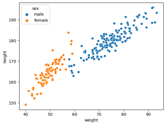
4. 적합
# step1 -- pass
# step2
predictr = TabularPredictor(label='height')
# step3
predictr.fit(df_train)
# step4
yhat = predictr.predict(df_train)
No path specified. Models will be saved in: "AutogluonModels/ag-20231221_040659/"
Beginning AutoGluon training ...
AutoGluon will save models to "AutogluonModels/ag-20231221_040659/"
AutoGluon Version: 0.8.2
Python Version: 3.8.18
Operating System: Linux
Platform Machine: x86_64
Platform Version: #38~22.04.1-Ubuntu SMP PREEMPT_DYNAMIC Thu Nov 2 18:01:13 UTC 2
Disk Space Avail: 650.40 GB / 982.82 GB (66.2%)
Train Data Rows: 280
Train Data Columns: 2
Label Column: height
Preprocessing data ...
AutoGluon infers your prediction problem is: 'regression' (because dtype of label-column == float and many unique label-values observed).
Label info (max, min, mean, stddev): (195.79716947992372, 148.97529810482766, 174.60543, 9.4301)
If 'regression' is not the correct problem_type, please manually specify the problem_type parameter during predictor init (You may specify problem_type as one of: ['binary', 'multiclass', 'regression'])
Using Feature Generators to preprocess the data ...
Fitting AutoMLPipelineFeatureGenerator...
Available Memory: 61087.3 MB
Train Data (Original) Memory Usage: 0.02 MB (0.0% of available memory)
Inferring data type of each feature based on column values. Set feature_metadata_in to manually specify special dtypes of the features.
Stage 1 Generators:
Fitting AsTypeFeatureGenerator...
Note: Converting 1 features to boolean dtype as they only contain 2 unique values.
Stage 2 Generators:
Fitting FillNaFeatureGenerator...
Stage 3 Generators:
Fitting IdentityFeatureGenerator...
Stage 4 Generators:
Fitting DropUniqueFeatureGenerator...
Stage 5 Generators:
Fitting DropDuplicatesFeatureGenerator...
Types of features in original data (raw dtype, special dtypes):
('float', []) : 1 | ['weight']
('object', []) : 1 | ['sex']
Types of features in processed data (raw dtype, special dtypes):
('float', []) : 1 | ['weight']
('int', ['bool']) : 1 | ['sex']
0.0s = Fit runtime
2 features in original data used to generate 2 features in processed data.
Train Data (Processed) Memory Usage: 0.0 MB (0.0% of available memory)
Data preprocessing and feature engineering runtime = 0.04s ...
AutoGluon will gauge predictive performance using evaluation metric: 'root_mean_squared_error'
This metric's sign has been flipped to adhere to being higher_is_better. The metric score can be multiplied by -1 to get the metric value.
To change this, specify the eval_metric parameter of Predictor()
Automatically generating train/validation split with holdout_frac=0.2, Train Rows: 224, Val Rows: 56
User-specified model hyperparameters to be fit:
{
'NN_TORCH': {},
'GBM': [{'extra_trees': True, 'ag_args': {'name_suffix': 'XT'}}, {}, 'GBMLarge'],
'CAT': {},
'XGB': {},
'FASTAI': {},
'RF': [{'criterion': 'gini', 'ag_args': {'name_suffix': 'Gini', 'problem_types': ['binary', 'multiclass']}}, {'criterion': 'entropy', 'ag_args': {'name_suffix': 'Entr', 'problem_types': ['binary', 'multiclass']}}, {'criterion': 'squared_error', 'ag_args': {'name_suffix': 'MSE', 'problem_types': ['regression', 'quantile']}}],
'XT': [{'criterion': 'gini', 'ag_args': {'name_suffix': 'Gini', 'problem_types': ['binary', 'multiclass']}}, {'criterion': 'entropy', 'ag_args': {'name_suffix': 'Entr', 'problem_types': ['binary', 'multiclass']}}, {'criterion': 'squared_error', 'ag_args': {'name_suffix': 'MSE', 'problem_types': ['regression', 'quantile']}}],
'KNN': [{'weights': 'uniform', 'ag_args': {'name_suffix': 'Unif'}}, {'weights': 'distance', 'ag_args': {'name_suffix': 'Dist'}}],
}
Fitting 11 L1 models ...
Fitting model: KNeighborsUnif ...
-3.463 = Validation score (-root_mean_squared_error)
0.21s = Training runtime
0.01s = Validation runtime
Fitting model: KNeighborsDist ...
-3.3929 = Validation score (-root_mean_squared_error)
0.02s = Training runtime
0.0s = Validation runtime
Fitting model: LightGBMXT ...
-3.0349 = Validation score (-root_mean_squared_error)
0.22s = Training runtime
0.0s = Validation runtime
Fitting model: LightGBM ...
-3.1331 = Validation score (-root_mean_squared_error)
0.16s = Training runtime
0.0s = Validation runtime
Fitting model: RandomForestMSE ...
-3.0811 = Validation score (-root_mean_squared_error)
0.29s = Training runtime
0.02s = Validation runtime
Fitting model: CatBoost ...
-2.8341 = Validation score (-root_mean_squared_error)
0.32s = Training runtime
0.0s = Validation runtime
Fitting model: ExtraTreesMSE ...
-3.0481 = Validation score (-root_mean_squared_error)
0.24s = Training runtime
0.02s = Validation runtime
Fitting model: NeuralNetFastAI ...
-3.0808 = Validation score (-root_mean_squared_error)
0.86s = Training runtime
0.0s = Validation runtime
Fitting model: XGBoost ...
-3.0563 = Validation score (-root_mean_squared_error)
0.27s = Training runtime
0.0s = Validation runtime
Fitting model: NeuralNetTorch ...
-2.8592 = Validation score (-root_mean_squared_error)
0.74s = Training runtime
0.0s = Validation runtime
Fitting model: LightGBMLarge ...
-3.1759 = Validation score (-root_mean_squared_error)
0.21s = Training runtime
0.0s = Validation runtime
Fitting model: WeightedEnsemble_L2 ...
-2.7259 = Validation score (-root_mean_squared_error)
0.15s = Training runtime
0.0s = Validation runtime
AutoGluon training complete, total runtime = 3.92s ... Best model: "WeightedEnsemble_L2"
TabularPredictor saved. To load, use: predictor = TabularPredictor.load("AutogluonModels/ag-20231221_040659/")[1000] valid_set's rmse: 3.05149sns.scatterplot(df_train, x='weight',y='height',hue='sex',alpha=0.3)
sns.lineplot(df_train, x='weight',y=yhat,hue='sex')<AxesSubplot: xlabel='weight', ylabel='height'>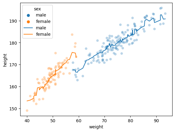
predictr.leaderboard(silent=True)| model | score_val | pred_time_val | fit_time | pred_time_val_marginal | fit_time_marginal | stack_level | can_infer | fit_order | |
|---|---|---|---|---|---|---|---|---|---|
| 0 | WeightedEnsemble_L2 | -2.725899 | 0.016733 | 2.555090 | 0.000230 | 0.151280 | 2 | True | 12 |
| 1 | CatBoost | -2.834127 | 0.000724 | 0.324964 | 0.000724 | 0.324964 | 1 | True | 6 |
| 2 | NeuralNetTorch | -2.859244 | 0.002492 | 0.736833 | 0.002492 | 0.736833 | 1 | True | 10 |
| 3 | LightGBMXT | -3.034869 | 0.001134 | 0.220292 | 0.001134 | 0.220292 | 1 | True | 3 |
| 4 | ExtraTreesMSE | -3.048093 | 0.018088 | 0.243790 | 0.018088 | 0.243790 | 1 | True | 7 |
| 5 | XGBoost | -3.056270 | 0.002459 | 0.271035 | 0.002459 | 0.271035 | 1 | True | 9 |
| 6 | NeuralNetFastAI | -3.080801 | 0.004651 | 0.863921 | 0.004651 | 0.863921 | 1 | True | 8 |
| 7 | RandomForestMSE | -3.081138 | 0.018505 | 0.294994 | 0.018505 | 0.294994 | 1 | True | 5 |
| 8 | LightGBM | -3.133082 | 0.000750 | 0.155065 | 0.000750 | 0.155065 | 1 | True | 4 |
| 9 | LightGBMLarge | -3.175914 | 0.000838 | 0.211776 | 0.000838 | 0.211776 | 1 | True | 11 |
| 10 | KNeighborsDist | -3.392890 | 0.004761 | 0.023989 | 0.004761 | 0.023989 | 1 | True | 2 |
| 11 | KNeighborsUnif | -3.463039 | 0.006178 | 0.207058 | 0.006178 | 0.207058 | 1 | True | 1 |
5. 해석 및 시각화
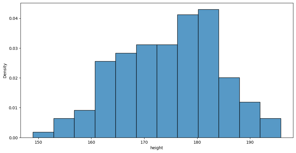
A. y의 분포, (X,y)의 관계 시각화
auto.target_analysis(
    train_data=df_train,
    label='height',
    fit_distributions=False
)
Target variable analysis
| count | mean | std | min | 25% | 50% | 75% | max | dtypes | unique | missing_count | missing_ratio | raw_type | special_types | |
|---|---|---|---|---|---|---|---|---|---|---|---|---|---|---|
| height | 280 | 174.605431 | 9.430102 | 148.975298 | 167.572671 | 175.186487 | 181.132612 | 195.797169 | float64 | 280 | float |
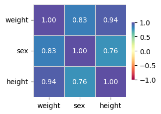
Target variable correlations
train_data - spearman correlation matrix; focus: absolute correlation for height >= 0.5
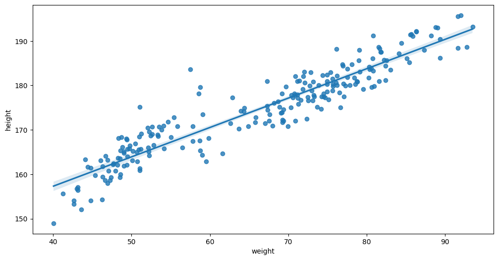
Feature interaction between weight/height in train_data
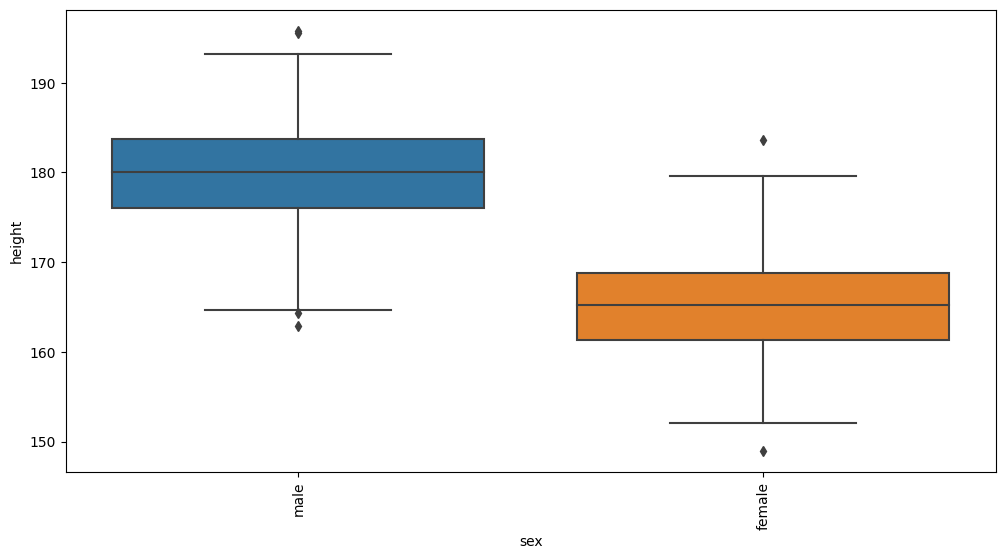
Feature interaction between sex/height in train_data
B. 중요한 설명변수?
- 중요하다고 생각하는 설명변수를 랭킹을 통해 알려줌
auto.quick_fit(
    train_data=df_train,
    label='height',
    show_feature_importance_barplots=True
)
No path specified. Models will be saved in: "AutogluonModels/ag-20231203_071354/"Model Prediction for height
Using validation data for Test points
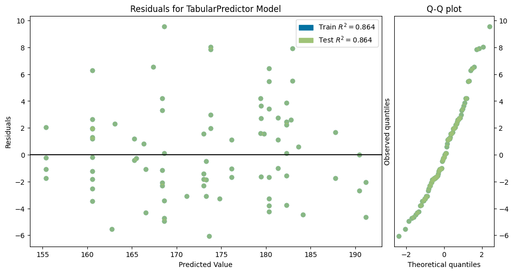
Model Leaderboard
| model | score_test | score_val | pred_time_test | pred_time_val | fit_time | pred_time_test_marginal | pred_time_val_marginal | fit_time_marginal | stack_level | can_infer | fit_order | |
|---|---|---|---|---|---|---|---|---|---|---|---|---|
| 0 | LightGBMXT | -3.441217 | -3.881789 | 0.006712 | 0.001602 | 0.306659 | 0.006712 | 0.001602 | 0.306659 | 1 | True | 1 |
Feature Importance for Trained Model
| importance | stddev | p_value | n | p99_high | p99_low | |
|---|---|---|---|---|---|---|
| weight | 9.433162 | 0.468715 | 7.290537e-07 | 5 | 10.398253 | 8.468071 |
| sex | 1.710680 | 0.464422 | 5.924364e-04 | 5 | 2.666932 | 0.754427 |

Rows with the highest prediction error
Rows in this category worth inspecting for the causes of the error
| weight | sex | height | height_pred | error | |
|---|---|---|---|---|---|
| 208 | NaN | female | 159.027430 | 168.600342 | 9.572911 |
| 263 | 54.145913 | female | 165.791300 | 173.811340 | 8.020041 |
| 146 | 76.642564 | male | 175.011295 | 182.954391 | 7.943097 |
| 228 | 56.473758 | female | 165.962051 | 173.811340 | 7.849289 |
| 92 | 51.018586 | female | 160.851952 | 167.398270 | 6.546318 |
| 198 | NaN | male | 173.915293 | 180.355164 | 6.439870 |
| 157 | 46.214566 | female | 154.289882 | 160.576065 | 6.286183 |
| 106 | 69.667856 | male | 179.665916 | 173.611328 | 6.054588 |
| 118 | 48.711791 | female | 168.305739 | 162.763138 | 5.542602 |
| 166 | 77.068343 | male | 177.439194 | 182.954391 | 5.515197 |
C. 관측치별 해석
0번 obs
- 0번 observation
df_train.iloc[[0]]| weight | sex | height | |
|---|---|---|---|
| 0 | 71.169041 | male | 180.906857 |
predictr.predict(df_train.iloc[[0]])0 178.642868
Name: height, dtype: float32- 왜 178.642868로 예측했을까?
- 해석
auto.explain_rows(
    train_data= df_train,
    model = predictr,
    rows = df_train.iloc[[0]],
    display_rows= True,
    plot='waterfall'
)| weight | sex | height | |
|---|---|---|---|
| 0 | 71.169041 | male | 180.906857 |
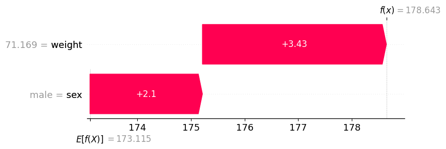
- 왜 178.642868로 예측했을까?
- 일단은 평균값인 173.115에 적합
sex을 고려하여 +2.1weight을 고려하여 +3.43- 최종적으로는 178.643
208번 obs
- 208번 observation
df_train.iloc[[208]]| weight | sex | height | |
|---|---|---|---|
| 208 | NaN | female | 159.02743 |
predictr.predict(df_train.iloc[[208]])208 168.788971
Name: height, dtype: float32- 왜 168.788971로 예측했을까?
- 해석
auto.explain_rows(
    train_data= df_train,
    model = predictr,
    rows=df_train.iloc[[208]],
    display_rows= True,
    plot='waterfall'
)| weight | sex | height | |
|---|---|---|---|
| 208 | NaN | female | 159.02743 |
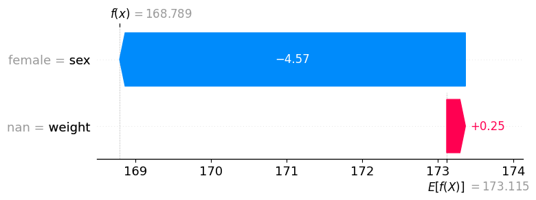
- 왜 178.642868로 예측했을까?
- 일단은 평균값인 173.115에 적합
sex을 고려하여 -4.57weight=nan을 고려하여 +0.25- 최종적으로는 168.789
결측치를 그냥 하나의 관측치로 해석함 (nan이라는 값을 가지고 있다고 해석하는 느낌)
이게 왜 가능한가? (이런걸 가능하게 하는 테크닉이 많음, nan을 -9999로 처리하고 트리를 돌린다고 상상)
211번 obs
- 211번 observation
df_train.iloc[[211]]| weight | sex | height | |
|---|---|---|---|
| 211 | NaN | female | 165.076235 |
predictr.predict(df_train.iloc[[211]])211 168.788971
Name: height, dtype: float32- 해석
auto.explain_rows(
    train_data= df_train,
    model = predictr,
    rows=df_train.iloc[[211]],
    display_rows= True,
    plot='waterfall'
)| weight | sex | height | |
|---|---|---|---|
| 211 | NaN | female | 165.076235 |

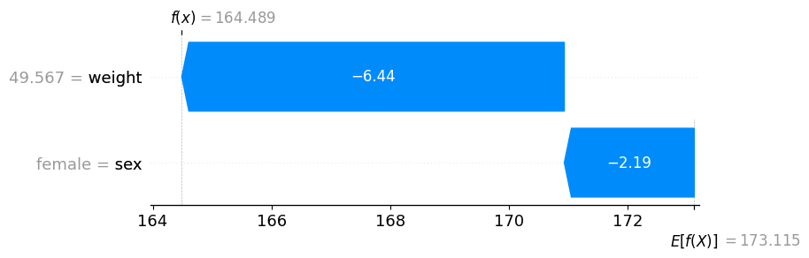
- 우리가 생각한 현실적인 적합은 사실 이러함
df_train[df_train.sex =='female'].weight.mean()49.567060917121516onerow = df_train.iloc[[211]].copy()
onerow.weight = 49.567060917121516
onerow| weight | sex | height | |
|---|---|---|---|
| 211 | 49.567061 | female | 165.076235 |
predictr.predict(onerow)211 164.488647
Name: height, dtype: float32auto.explain_rows(
train_data= df_train,
model = predictr,
rows=onerow,
display_rows= True,
plot='waterfall'
)| weight | sex | height | |
|---|---|---|---|
| 211 | 49.567061 | female | 165.076235 |
198번 obs
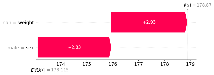
- 198번 observation
df_train.iloc[[198]]| weight | sex | height | |
|---|---|---|---|
| 198 | NaN | male | 173.915293 |
predictr.predict(df_train.iloc[[198]])198 178.869781
Name: height, dtype: float32- 해석
auto.explain_rows(
    train_data= df_train,
    model = predictr,
    rows=df_train.iloc[[198]],
    display_rows= True,
    plot='waterfall'
)| weight | sex | height | |
|---|---|---|---|
| 198 | NaN | male | 173.915293 |